
Raspberry Shake to Go – an HVSR Adventure
Published on October 9, 2025
By Riley James Balikian
Introduction
Riley Balikian works as a geophysicist and hydrogeologist at the Earth Characterization Center (ECC) in the Illinois State Geological Survey (ISGS), part of the Prairie Research Institute (PRI) at the University of Illinois-Urbana Champaign (UIUC). The data they collect with their portable seismometers and the information derived goes directly into maps and models depicting the depth to bedrock beneath the glacio-fluvial sediments that drape the surface through much of Illinois. These seismic data are used to define and refine bedrock surface topography especially, which is a significant control on the availability of groundwater for municipalities, farms, homes, and businesses throughout the state.

ISGS student intern acquiring data using a Raspberry Shake near downtown Chicago, at planned future site of the Chicago Fire MLS stadium
I had never heard the term “honey wagon” before my colleague informed me that one had run over our portable Tromino seismometer (as I soon learned, a “Honey wagon” is a euphemistic term for a truck that empties portable toilets). For all practical purposes, seismic data acquisition for our summer field season was all but flushed.

Our broken Tromino seismometer
Though we still had one Tromino instrument, using a single seismometer would severely limit the number of data points we could collect on a field excursion, which significantly increases costs and decreases the amount of data we can acquire on a project.
We needed a new portable seismometer if we were to be able to expeditiously continue our work characterizing the shallow subsurface in Illinois, and soon. The funding that allows us to carry out our investigations often disappears in a matter of months, even if the geology we seek to understand remains unchanged.
Geologic Context
The furthest southern-reaching glacial ice sheet of the Pleistocene (the geologic epoch that lasted from about 2.6 million years ago until about 12,000 years ago) in the Northern Hemisphere stopped its advance in the southern tip of Illinois. (This glaciation is referred to as the “Illinoisan” because of this fact).
From this and other glaciations, most of the surface of the Illinois is covered with sediments deposited by glaciers and glacially-swollen rivers. Because of this, one of the most important buried geologic interfaces we try to keep track of is the topography of the bedrock. In some places, the bedrock surface and the ground surface are the same. Indeed, in the more scenic regions of the state–Garden of the Gods, the Driftless Region, Starved Rock, Mattheissen State Park, and along the Mississippi River–the bedrock is the defining feature of the landscape.
In most places in Illinois, however, the landscape at the surface is relatively flat, glacially-deposited sediment as far as the eye can see. These sediments are composed of sands, gravels, clays, boulders and various mixtures thereof, packed down by ancient glaciers of unspeakable height.
These glacial sediments and the soils built from them are what enabled the flourishing of the eponymous prairies of the Prairie State. In some places in Illinois, where thick glacial sediments were laid down in preexisting valleys in the bedrock, these unconsolidated layers of glacial sediments can reach nearly 600 feet deep. Until about the 1960s, the tallest buildings in Chicago could have been completely buried in the state’s deepest valleys of glacial sediment.
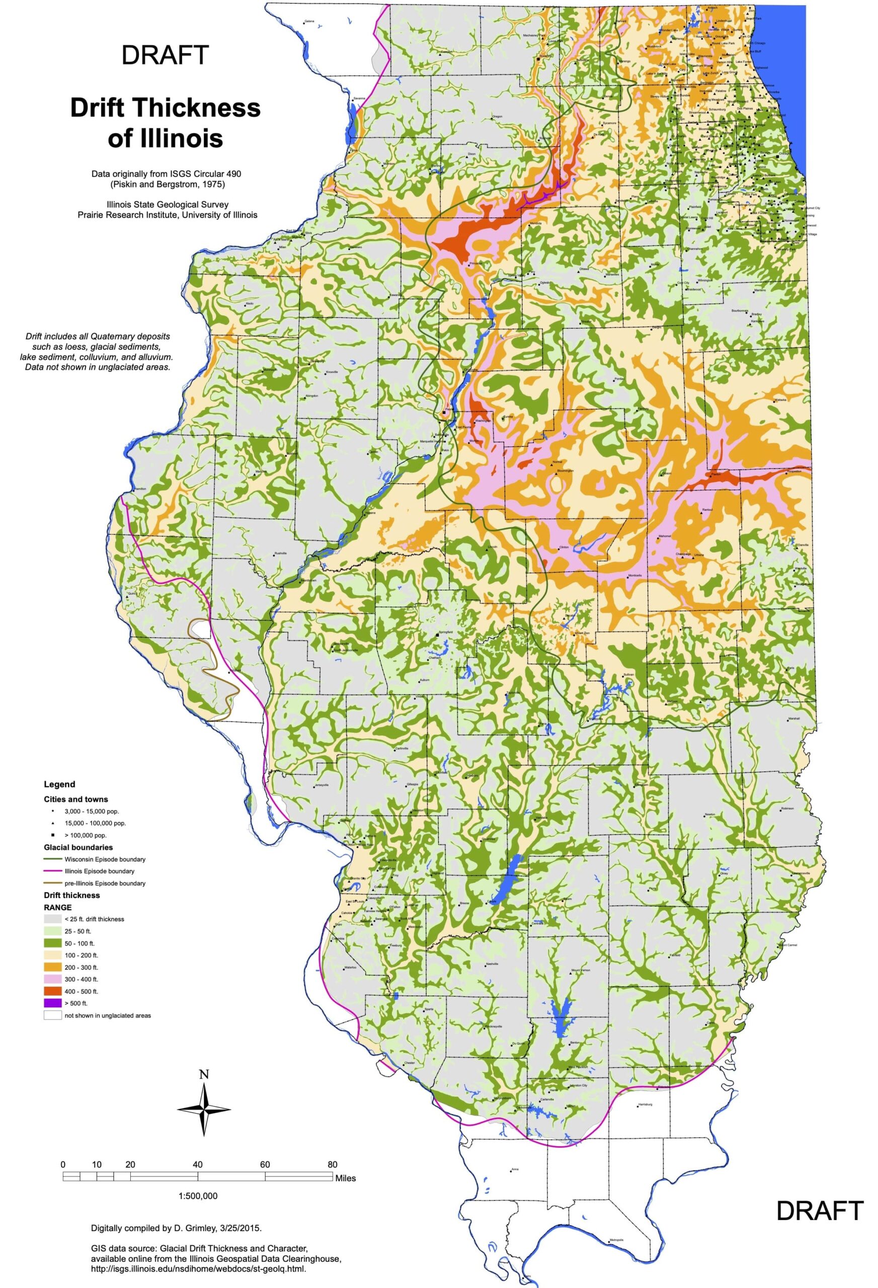
Map of the thickness of glacial drift in Illinois
How we use our seismic data
Resonances of the past
The contours of bedrock valleys and other buried bedrock features are often among the largest unknowns when it comes to creating geologic maps, groundwater flow models, and other near-surface geologic products for public consumption in Illinois.
There are two primary ways we can gather data about buried bedrock features: 1) drill wells, or 2) use geophysical data. Drilling wells is fairly expensive. It requires multiple highly trained individuals operating large, expensive equipment in complicated terrains over the course of several days or weeks. While it gives us a highly detailed understanding of the stratigraphy at that location, it also only provides a single depth to bedrock at a single location.
If bedrock topography is our main concern, geophysical data can decrease the cost of data acquisition by an order of 1000 and can expand and extend our understanding beyond a single site. However, many of the near-surface geophysical techniques we use do not reliably penetrate to the depths needed for those deepest bedrock valleys. With some of our electrical geophysical methods, we can also run into issues where glacial sediments and bedrock formations do not differ significantly enough in their electromagnetic signatures to distinguish them in the data. This is where we bring in our portable seismometers.
Our portable seismometers are deployed most commonly with the intent to acquire ambient seismic data and to process the data using the Horizontal to Vertical Spectral Ratio (HVSR) technique. The HVSR technique takes advantage of the physical phenomenon in which seismic waves–specifically the horizontal component of surface seismic waves–resonate at a fundamental frequency associated with an acoustically-significant subsurface boundary (often, the interface between unconsolidated material and bedrock). The vertical component of these waves do not resonate to the same extent. So, at that resonant frequency, the spectral power recorded by the horizontal components of a seismometer will be significantly higher than the power at that same frequency recorded by the vertical component. By calculating the ratio between the power of the seismic waves in different planes and at different frequencies, a fundamental frequency for a specific site can be estimated with just a single seismometer and with ambient seismic data.
HVSR was developed in the 1970s and 1980s in Japan as a somewhat unexpected secondary result of work to create an earthquake early warning system for railroads and to carry out geotechnical site characterizations for the building of various structures in that country.
With the frequency and strength of earthquakes in Japan, understanding how a site might respond to these impulses remains an important consideration in the construction of high speed railroads and other infrastructure there. (HVSR is also called the “Nakamura method” after one of the scientists working at the time at the Railroad Technical Research Institute who helped prove and explain the theory and many of the limitations behind the phenomenon that HVSR uses).
Since then, the most important advances in HVSR were borne from the SESAME project in Europe in the early 2000s (SESAME stands for Site Effects aSsessment using AMbient Excitations). The SESAME group carried out numerous tests to better understand the theory behind HVSR, the instrumentation used in HVSR measurements, and the software and statistical analyses used to formalize and standardize the processing algorithms used in HVSR. They published software, articles, and some of the best-practices for data analysis that are still in widespread use today.
Both before and since the SESAME project, HVSR has been used in many different environments and for many different purposes. Because HVSR can be used with a single seismometer, it is one of the few geophysical techniques taken from direct measurements on the Earth, the Moon, and Mars. In any case, the work of SESAME, Nakamura, and other scientists before and since have made HVSR viable as a scientific method, and enabled the development of software and hardware oriented towards the HVSR method.
The image below shows a typical result we get from processing HVSR data from an ambient seismic record using the SpRIT HVSR processing software (this site was recorded using a Raspberry Shake).
When we process data, we typically break our 20-60 minute dataset into windows (often, 20-60 seconds each). For each of these windows, we calculate a power spectral density (PSD) curve. Often, we end up with 80-200 windows, and therefore 80-200 curves. These curves are averaged on a per-frequency basis to provide the “primary” curve for each component (and eventually, the primary HVSR curve). Because we have dozens of curves, we are able to calculate statistics such as the standard deviation of the measurement for each frequency bin. The standard deviation, for example, is displayed as a semi-transparent area behind each primary curve in the report figure below.
In this HVSR report, the top chart represents the “primary” H/V curve that is used for analysis. This represents the ratio of the power at each frequency between the combined horizontal components and the vertical component. The middle chart shows the power spectral density curves for each component (the red and blue are averaged, then divided by the black to give us the top chart).
The bottom chart is a different way of displaying the top chart, but instead of representing the many input curves simply by their standard deviation, the amplitude of the H/V curve is depicted by color, the Y axis is frequency (as if the top curve was turned on its side) and the x-axis is time. This allows us to visualize the stability of the H/V curve over time. When our data is nice and cooperative (as in the displayed report), we often see a bright horizontal line at the fundamental frequency throughout the entire record.

Example results from HVSR processing of ambient seismic data using the SpRIT HVSR Python Package
Raspberry Shakes for HVSR
Our portable Tromino seismometer, which was run over and destroyed a few years ago, is an instrument built and marketed specifically for use with the HVSR technique. It is considered by many to be the “industry standard” equipment for HVSR. Though not expensive relative to some of the other geophysical equipment we use at the ISGS, it is nevertheless about 5x more expensive than a Raspberry Shake.
In researching whether the Raspberry Shake could adequately perform rigorously enough for our scientific endeavors, we found a recently published paper comparing the output of the Raspberry Shake 3D to a Nanometrics Trillium Compact 20s seismometer–a seismometer that ostensibly would have greater precision than even our recently-defunct portable seismometer.
The results of that article, in summary, show that while the Trillium seismometer does a better job at recording seismic signal over a very broad range of frequencies, the Raspberry Shake 3D would likely perform adequately for our purposes in the frequency ranges of interest (the vast majority of the data we’re interested in is between ~0.7 Hz – 30 Hz). So, we were able to borrow a Shake from a colleague and put it to the test in field conditions.
Thus far, a qualitative summary of the performance of the Raspberry Shake 3D for HVSR in Illinois environments is that it performs adequately and without noticeable degradation in the HVSR curve most of the time. In the deepest bedrock valleys in Illinois, where the bedrock is greater than 500’ (150 m) in depth, we do notice that the more expensive instruments tend to have fewer issues with respect to signal to noise ratio in the lower frequencies (this is in agreement with the findings of the previously-mentioned manuscript). Even so, the greatest variability tends to be less due to the kind of instrument deployed and more due to the specific geologic/ambient noise conditions at the site.
Raspberry Shakes in HVSR Practice
Project Planning
After having used a Raspberry Shake 3D for one (half of) a field season, we decided to move forward with the purchase of additional Raspberry Shakes for future seasons. As we did this, we needed to think in more detail about how the Shakes are used in practice over the entire “HVSR project lifecycle”. This involves many steps including project planning, instrument staging, data acquisition, data extraction, data management, data analysis, and reporting of results.
One somewhat unique aspect about the way we function at the ISGS is that we have a fresh batch of primarily undergraduate student staff who join us each field season to help with data acquisition. So, for each step of the HVSR lifecycle, we needed to make sure it was feasible for these students to carry out the necessary tasks. The students who work with us often have just an introductory level of experience with geology or geophysics and even less experience with computer science and geophysical instrumentation. So, if the Raspberry Shakes were to be viable field instruments in practice, it was essential for their deployment to be characterized by a simple user experience.
Below is a table summarizing how we conceptualize the HVSR lifecycle steps, comparing between Raspberry Shakes and other more established instruments used in the field:
| HVSR Step | Established HVSR instrument(s) | Raspberry Shake 3D |
| Project Planning | Minimal cultural noise; need a location to site instrument | |
| Instrument staging | Some instruments require extra device Standard batteries (e.g., AA) Single device; no external accessories | Additional device needed (e.g., laptop) 12V battery and custom voltage converter Multiple cables and plugs needed |
| Data Acquisition | Long setup procedure in field | Simply turn on device and ensure timing is correct; notes for timing are important! (or use HVSR script detailed below) |
| Data Extraction | Dedicated software needed (often with expensive licensing) | Can be done with terminal commands or free 3rd party software |
| Data Management | Data may be in proprietary format | Data in standard seismic format (MiniSEED) |
| Data Analysis | Often, dedicated software needed | Open source or other HVSR software needed (we use/developed SpRIT python package) |
| Reporting of Results | Limited to outputs provided by software | Flexible with whatever outputs you produce |
Hardware Updates
The available formats for the Raspberry Shake instruments are not really conducive “out of the box” to the way we collect HVSR data. Usually, we deploy an instrument for 20-60 minutes at a site, before moving it to a new location. This is done in remote field locations. The indoor acrylic enclosures provided by Raspberry Shake are not rugged enough for this type of treatment, and the IP67 plugs on the outdoor enclosure are intended for permanent deployment, and not rapid plugging/unplugging (we broke multiple ports in a single field season just by regular use).
Fortunately, the Raspberry Shake setup is fairly flexible, especially with the DIY kit. So we sought to emulate the portability of the more standard/commercial instruments while retaining the flexibility advantages offered by the Raspberry Shakes. In short, we needed some hardware modifications.
The simplest hardware modifications we undertook were to replace the somewhat cumbersome IP67 ports on the outdoor enclosure for ports that could be more regularly and easily plugged and unplugged. For example, we installed standard USB and ethernet ports (with IP67 covers) on the outside of the standard Shake outdoor enclosures, and installed a 12V-5.1V converter on the instruments themselves. These are not as weatherproof as the standard Outdoor enclosure (though we have plans to fix that), but we also do not collect data in inclement weather. Over multiple field seasons, these have not given us any issues yet, though we tend not to acquire data in inclement weather. We also have been trialing a completely enclosed system that will be described in more detail below.

Updated ports and voltage converter (12v-5v) on the HVSR outdoor enclosures. While the ports themselves are not as weatherproof as the included ports, the covers have the same IP rating and they work much more seamlessly with our workflow. The voltage converter also has a cover/case that is not pictured.
Software Updates
On the software side, it also made sense to add some functionality both on the instrument itself and in the processing of the data, which is only possible because of the relatively open-source implementation of the Shake OS on Raspberry Pi systems. These updates involved changes in the "firmware" of the Shakes as well as software for using and processing acquired data.
For processing HVSR data, the Incorporated Research Institutes for Seismology (IRIS) (IRIS is now called Earthscope) have developed a Python package for carrying out HVSR analysis on the instruments and data available via their MUSTANG web services (specifically, the noise-psd web service). The MUSTANG noise-psd service provides power spectral density (PSD) calculations on seismometers in their networks. These pre-calculated PSD values are what are fed into the IRIS HVSR python library. The IRIS HVSR library took these PSD data, and carried out HVSR analysis. We built off this library by adding in algorithms to calculate the PSD values and otherwise prepare raw seismic data on a specific device (for example, as extracted from a Raspberry Shake on a laptop). We developed a new python package called SpRIT that can process data from a 3-component seismic file readable by the well-established Obspy python package, or which can interface cleanly with the BUD-like file structure (////{MSEED DAY FILE) on the Raspberry Shake itself to extract a single, site-specific 3-component MiniSEED file. SpRIT also produces a data object that can be post-processed for further analysis beyond simple HVSR calculations, including the creation of depth curves and HVSR cross sections.
For "firmware" on the Shake itself, we developed what we eloquently call "the Shake HVSR script" that can be run as a standard terminal command (via SSH) on the Shake, which tells the Shake to acquire data for a specified amount of time, combines the 3 streams into a single file for that time window, outputs the data to a MiniSEED file saved in a specified directory on the shake, and gracefully powers down the Shake so it can be moved to the next location without accessing the instrument via SSH a second time. Though it requires no significant change in the OS software, it does require the installation of the "screen" terminal tool (sudo apt install screen) to continue running on the Shake after the SSH device has been disconnected.

Example output while running the HVSR script on the Shakes
These simple changes have made the Shakes easier to use and superior in many ways to more expensive, commercially-marketed seismometers for the purpose of collecting HVSR data.
The current HVSR lineup

The HVSR family photo, showing our current HVSR instrumentation array consisting of 3 Raspberry Shakes in standard outdoor enclosures, 1 portable Shake, and 1 Tromino
Currently, for HVSR deployment, we have three of the slightly modified outdoor Shakes (“Rachel”, “Hagrid”, and “Debbie”), the remaining Tromino instrument (“Trey”), and the highly modified portable Raspberry Shake To Go (“Rita”). (Our students have, over the years, given each of the instruments nicknames based on their station code.)
While we have not yet carried out a complete quantitative comparison of the data between the different instruments, we have acquired a handful of sites with all 5 instruments (we are also currently renting a Nanometrics Trillium Compact 20s that we also hope to compare in the field). The figure below is a representative comparison of the HVSR results from these instruments (this site is the one pictured above in the “ISGS HVSR Family Photo”).
Of note, the three Shakes in the outdoor enclosure exhibit remarkably similar results. The Tromino also has similar results throughout the H/V curve, but interestingly, the amplitude of the peak resonance is lower than that of the Shakes (I would expect higher-quality instruments to potentially have clearer resonance). The frequency of the peak resonance at this particular site is a slightly higher frequency on the Tromino (though within a standard deviation). The noise in the H/V curve in the lower frequencies appears to be more attenuated by the Tromino than the Shakes. Rita (our portable version of the Shakes) experiences a smaller peak, but it has a remarkably similar peak frequency as the other Shakes, which themselves are in good agreement with each other.
I do want to investigate further whether the seeming slight, upward shift in peak frequency at this site by the Tromino from the Shakes is persistent, but this otherwise shows encouraging results as to the replicability of the measurement between different instruments and instrument types.

HVSR results at single, representative site for 3 Raspberry shakes in standard outdoor enclosures (“Hagrid”, “Debbie”, and “Rachel”), 1 portable shake (“Rita”), and 1 Tromino system
A Portable Raspberry Shake Seismometer
Having used Raspberry Shakes in modified outdoor enclosures for the past two field seasons, we have more confidence now in their ability to provide the kind of data we need for HVSR analysis in Illinois. This has allowed us to experiment with their setup. We bought a DIY Shake kit that we have heavily modified for this purpose, which is explained in detail below.
If necessity is the mother of invention, some of the constraints from the standard outdoor enclosure is what has guided much of the development of our portable Raspberry Shake Seismometer. We also wanted to make it replicable so that it did not require intricate circuit design or inordinate amounts of permanent modifications. In short, we wanted most parts to be “off the shelf” and the steps to be fairly straightforward. We also used some of the same modifications we had already implemented on the other outdoor enclosures (e.g., IP67 covers on regular ports).

Casing, power button, and ports for the portable shake. On opposite side of casing (not pictured) are latches and a removable SD card access port, which is an electrical enclosure plug inserted into plastic casing by heating the metal plug and melting it into the plastic
Power supply

PiPower module (black circuit board) in Portable shake. USB-C input connects to external USB-C charging port. USB-A output connects with MicroUSB input to Raspberry Pi Model 3
For example, one of the first things we attempted to increase portability was to enclose a power source in the Shake. This has proven to be the most tedious obstacle to overcome in creating a portable Raspberry Shake seismometer, though we believe we have a workable solution.
Because the Shake’s “hat” covers most of the Raspberry Pi GPIO pins, many standard power modules (and other add-ons, for that matter) for Raspberry Pi’s could not be used alongside the Shake. Also, the Raspberry Pi models compatible with Raspberry Shakes need to have power capabilities slightly exceeding most standard 5V devices, rendering many of the power sources for other 5V devices unusable.
We eventually found the Sunfounder PiPower module, which powers the Shake via its standard USB power input (either micro USB or USB-C depending on the model). It also has the ability to be controlled by an external power button, so could be attached inside an enclosure while still being accessible from the outside. With the provided 2x 18650 batteries, we have found that it provides about 5 hours of power in ideal conditions before it needs to be recharged. We usually only collect 20-60 minutes at a time, so this works for us. There is also an option to add additional batteries to this module, and a standard powerbank can be used to pass power through the PiPower module, further increasing the flexibility of the instrument.
It is not a perfect solution–during initial testing, there was occasionally a voltage issue during boot in which the Shake inexplicably entered a boot-loop even though the voltage was ostensibly high enough for regular function. But we have addressed many of these issues in our latest iteration of the setup procedure, and have been able to use this in the field most of the time with no issues.
Wireless Connectivity

Wifi dongle as mounted on right angle USB for easy access and potentially better reception on portable shake
We also wanted the Shake to ideally be usable wirelessly in the field. For SSH connections, it is necessary for the device accessing the Shake to be on the same network as the Shake itself. We often bypass this in the field by directly connecting an Ethernet cable between the Shake and our laptop.
However, a wireless connection would improve usability and would eliminate seismic interference during the acquisition record by an operator approaching and handling the instrument. Since it would not require a direct ethernet connection, it would also allow phones, tablets, and other devices to be used (via the rs.local dashboard or using SSH via the, e.g., termux app) to check in on and gracefully power down the instrument at the end of acquisition for a particular site. Creating a wifi connection would be an ideal solution.
Creating a wireless connection to the Shake in the field was actually our first attempt at “updating” the hardware, and within a few weeks of acquiring our Shake, we actually had it working quite well in field conditions. A relatively minor obstacle to simple use of the wifi on the Raspberry Shake is that the internal wifi module on the Raspberry Pi generates too much radio frequency noise to be used during data acquisition.
However, this is fairly easy to overcome: adding a USB wifi dongle allows us to have wifi connectivity while also collecting data. A quick online search will show that there are a myriad of low-power Raspberry Pi-compatible wifi dongles available. It seemed to us that one of the more simple ones to use “out of the box” would be a dongle using a mediatek chipset (see here). We do have to “install” the firmware (i.e., transfer the mt7601u.bin file available for download here (downloaded by clicking the “plain” button) to the /lib/firmware directory on the Shake), but then it works without issues.
Now that the Shakes had wireless capability, we just needed a network to connect them to. Because we are often in remote locations in the field, internet access (even via cellular technology) is not always possible. But, we quickly surmised that a connection to the world-wide web is not required…any old network will do!
So, we experimented with relatively old, used mobile hotspots we found on eBay. While these would not connect to the wider internet without an active subscription (and were perhaps too old and outdated even for that), they could easily create a local network that both the Shake and our laptops could connect to. This would allow them to connect via SSH at a distance large enough so that an operator would not interfere with the data itself. We could even download data wirelessly! After our first week of use, we were impressed with how simple and streamlined this wireless solution was.
Or, so it seemed.
The GPS conundrum

Picture of Sparkfun GPS module (small red chip) with wires to portable Shake. Note the Sparkfun GPS module also allows addition of an external GPS antenna (picture on the right of the casing), though the specific antenna in use does not appear to enhance the reception greatly in tests beyond the square ceramic antenna included on the chip itself
Upon examining the data from that week, there were numerous, unexplained gaps and overlaps in our data, rendering it essentially useless for analysis. Upon further examination, the culprit appeared to be the USB GPS device. From the online Shake forums and the technical manual, it was confirmed to us that the provided USB GPS device needs exclusive access to the USB ports on the Raspberry Pi to work effectively. Because we are in remote locations, GPS is necessary for timing, and timing is among the most important dimensions of the data for HVSR and other seismic analysis. So much for our wireless connection. We abandoned the hotspots in favor of the GPS antenna functioning properly.
Having seen how well the wireless connection could work and enhance our field process, I very much wanted to find a solution that would allow both wifi and GPS to be used in tandem. The GPS solution provided with the Shake that uses a “mouse” style USB antenna is workable, but I wanted the Shakes to be as nimble and easy to use as possible. Because of their demand for exclusive USB use, a non-USB GPS device was the logical choice for a solution.
Upon searching for standard Raspberry Pi GPS modules, we ran into several difficulties: most of them either a) use a “hat” interface to the GPIO pins (and therefore are not physically compatible with the blue Shake circuit board) and/or b) use serial interfaces that would either directly interfere with the incoming data from the geophones or would otherwise be quite difficult to program. There seemed to be a potential for bit-banging raw GPS streams through the few open GPIO pins, but this seemed likely to be too specific for widespread use, too time-demanding to develop, and might put undue strain on the Raspberry Pi itself.
One workaround for this was to find a GPS module that interfaces via i2c and which has PPS capability. There are a few of these available on the market, though they are not nearly as plentiful as those that use the standard UART interfaces.
We found a Sparkfun GPS Breakout module that met these requirements (we have not tested the PiMoroni PA1010d module since it has been out of stock, but it also may work). This required some creative solutions for reading in GPS data and (an unexpectedly difficult step) for using that GPS data to update the system time. (LLMs were very helpful in fine-tuning some of this work).
Our first attempt included parsing the input GPS stream via a Python script that then fed NMEA-formatted strings into GPSD. (GPSD is the “daemon” or background service that handles GPS data). This was actually not too difficult as a step: after the Python script was created, we just needed to change the GPSD configuration file (an unexpected issue was that the GPSD configuration file always resets on startup, so we had to set the file as “immutable” for it to continue to function properly). We were able to confirm the GPSD was reading the parsed data correctly using the cgps command and gpsmon command.
What proved to be more difficult was having GPSD transfer the GPS (specifically, timing) data from the GPS input to the timing service. Our initial solution involved creating a background service that creates a virtual terminal that uses shared memory between GPSD and NTPD (the timing service/daemon) to get timing data from the GPS into the system time. There seemed to be issues with user permissions and several other little things that kept popping up that prevented this from working properly. So we took a few steps back and tried a different approach.
The timing daemon that ships with the Raspberry Shake OS is NTPD. While it is possible that a solution could be created using NTPD, online forums and other sources seem to indicate that another timing service called chrony works better when there are large gaps between timing updates. Since we are constantly turning off and on our Shakes at different sites, this seemed to be an important feature. It also had (in our opinion) a slightly easier method for fine-tuning timing sources. So, we also installed chrony on our device to handle timing. We also installed separate PPS tools for handling the input PPS Data.
In the end, with a little more research on ways to bypass user permission issues and to ensure the timing data is fed into the system time with as little lag or latency as possible, we tried a different approach (outlined here) that uses a “named Pipe” (or First In First Out interface) to “stream” the GPS data to the GPSD daemon and separately uses the PPS input to help achieve nanosecond-scale timing precision. This seems to work quite well and we have now used it for about half of a field season, though we are still testing to make sure it works in as many use cases as possible.
Finally, there were a few hardware issues to resolve once the software was all figured out. First, our solution requires hardwiring/soldering a few cables to the back of a few unused GPIO pin ports on the blue Raspberry Shake board itself, which is admittedly not an ideal modification. We also found that we had to revisit the power supply issue, and had to fine-tune the power demands by turning off a few unused, higher-demand background components to ensure the Shake runs continuously without entering a boot loop.
However, with this in-place GPS solution, we both have a more contained instrument, and the ability to use our USB ports again for a wifi dongle. We have also found that we can use our USB port to export data in addition to the SSH connection. In the few tests we have carried out, the GPS/PPS solution appears to have temporal accuracy on the order of tens of nanoseconds.
All together now
With all of these components in place, we needed to find and build a suitable enclosure. This has not been too difficult, but it required many steps and lots of planning. We are also fortunate to have access to some tools that others may not.
Thus far, we have been using the Zulkit 5.9” x 5.9” x 3.5” enclosure. Fortunately, a library near our office allows access to a laser cutter, and we were able to adapt the .dxf file provided by Raspberry Shake using Inkscape to ensure the dimensions were correct to precisely, quickly, and affordably laser cut a bottom plate that both allows mounting the geophone and shake/pi boards as well as connecting all the components securely to the enclosure.We needed to use a thread tap to cut threads into the acrylic.
For now (this is likely a future area of improvement), we have used threaded inserts that are melted into the corners of the enclosure to mount the legs (something akin to these components). Our legs are essentially M5 stainless steel bolts that we cut to size. Since we are pushing the legs into the dirt, it is ok for our use case that there are four legs instead of the more ideal three legs. Eventually, a solution like the outdoor enclosures that have a firm bottom plate beneath the enclosure would likely be a useful addition.
Finally, we have used various IP67 panel mount ports for USB, Ethernet, power button, charge port, and access port for the microSD card containing the operating system. Our “cheap” way of installing these ports (without a proper and expensive die-cutting system) is to simply use a soldering iron to melt the holes in the correct shape through the enclosure. Dirty and inelegant, but it seems to work well enough, if not perfectly.
With these hardware and software modifications, we have been able to collect many times more data than previously. In one of the field seasons since our adoption of Raspberry Shakes for HVSR, we had three different teams collecting quality HVSR data in the Chicago area, Central Illinois, and Northern Illinois at the same time–a feat that would not have been possible for us just three years ago. The data we have collected has informed the interpretation and mapping of bedrock topography, which in turn has enabled us to better delineate glaciofluvial aquifer systems that serve as water sources and recharge zones for hundreds of thousands of Illinois residents. We are using the HVSR data we collect with Raspberry Shakes and other systems in conjunction with a myriad of other data sources to better understand the world beneath our feet.

Image of a deployed portable shake with its lid open for ease of view
Recipe for a Raspberry Shake To Go
The “recipe” for the setup described in this article is below:
Ingredients:
- Raspberry Shake 3D (DIY kit ok)
- Raspberry Pi (we have been using Model 3 (DYI kit does not come with Pi))
- Zulkit 5.9” x 5.9” x 3.5” enclosure
- Sunfounder PiPower UPS Module
- Acrylic sheet cut to size (this works with the Zulkit enclosure)
- M2.5 standoffs of various sizes
- Panel mounts or ports:
- USB-C (for charging PiPower)
- Ethernet
- USB
- Toggle Button
- Access port (electrical box enclosure plugs, installed by melting with soldering iron into plastic (creates its own threads)
- Solder, soldering iron, and various lengths of small-gauge wire
- Optional: Wifi dongle (ours with mediatek chipset here; driver here)
- Optional: i2c compatible GPS module with PPS capability (our Sparkfun module here)
- Otherwise, the standard USB GPS antenna from Raspberry Shake works (but then no wifi)
Instructions:
- See Tinkercad model here for a general setup that works for us.
- In this model:
- Orange cylinders = geophones
- Blue cylinder = USB panel port
- Yellow cylinder = ethernet panel port
- Red cylinder = latching power button
- Black cylinder = USB-C charging port
- Green board = Raspberry Pi
- Blue board = Raspberry Shake “hat”
- Black board = PiPower “hat”
- Batteries mounted on acrylic sheet beneath raspberry pi
- GPS board mounted on top of PiPower “hat”
- In this model:
- HVSR Script setup instructions see here
- GPS software setup instructions see here
- General initial setup instructions for our shakes here
As far as we can tell, this portable setup may introduce some noise or slightly diminish the seismic signal that is read into the Shake itself. So far, it has been usable in most cases, but it may not be as broadly usable as the Shakes bought directly from the manufacturer. The main difficulty for all of this is that the Raspberry Pi’s that are compatible with the Shake OS require a lot of power, and these power constraints put the portable system at a distinct disadvantage out of the gate with the more professional/commercial systems otherwise used for HVSR analysis.
With that said, the Raspberry Shakes are the backbone of our HVSR program, and have enabled a rapid expansion of the acquisition and analysis of ambient seismic data for HVSR processing around the state. This has helped us find and confirm the locations of previously unmapped bedrock valleys and their tributaries, enhancing the inputs to hydro-geologic models and maps in Illinois.
Acknowledgements
Thanks go out to several students, interns, and staff at ISGS and University of Illinois for their help getting these Shakes ready for field use. Specifically, thanks to Dr. Sherilyn Willams-Stroud for her lending of the initial Raspberry Shake we modified for HVSR use, Steve Sargent for coming up with, testing, and implementing most of the power supply modifications, Yesennia Nicacio-Rosales for her work on hardware and software modifications, Aman Jhurani for his work on software modifications, Steven Young for leading field acquisition of much of the ambient seismic data for the Shakes and comparable instruments, and Dr. Jason Thomason for the willingness to use and experiment with new instrumentation on projects for which he was the Principal Investigator. Others who aided with acquisition of data or the HVSR processing workflow in general include (but are not limited to): Dr. Timothy Larson, Alexx Sanchez, Dr. Hongyu Xiao, Emma Weber, Dr. Mitchell Barklage, Nicte Rivadeneyra-Braswell, Nick Karahalios, Anne Matson, Shaina Lohman, Preston Kietzman, Matthew Huisman, Kara Fowler, Devin Durica, Preston Howell, Avriel Mentado, Daniel Chukwudi, Nyla Williams, Aiden Fanning, Alex Riley, Lilly Drager, Lani Kiene, and Caleb Ortman.

Riley Balikian, author of post, acquiring geophysical data at a the Cahokia Mounds World Heritage Site in Illinois