Things you might find with your Raspberry Shake – Part 2
May 27th, 2026
by Alan Sheehan and Philip Peake
(More examples to help identify what you are seeing)
If you’re approaching this series for the first time, we recommend starting with Part 1, which covers earthquake detection and background-noise fundamentals. It’s also worth reading the Raspberry Shake Basic Concepts guide if terms like EHZ, HDF, helicorder, or spectrogram are new to you as we’ll be using them throughout.
Earthquakes are only one category of signals your Raspberry Shake can detect. Once you become familiar with seismic wave patterns and everyday background noise, a much wider world of signals starts to emerge.
Some come from human activity, for example:
- aircrafts
- quarry blasts
- rockets
- electrical interference
- industrial operations
Others, instead, originate in the natural world around us, such as:
- lightning
- sonic booms
- meteors
- volcanic shock waves
- and even re-entering space debris(!)
At first glance, many of these signals can look confusingly similar to earthquakes. Some produce sharp impulses, others generate long, low-frequency traces, and a few create patterns that are unlike anything geological at all.
In this second part of the series, we’ll explore some of the most recognizable non-earthquake signals seen on Raspberry Shake stations and how to distinguish them from genuine seismic events.
Aircrafts
Helicopters
Helicopters are among the easiest aircraft to recognize on a Raspberry Shake. Unlike fixed-wing aircraft, helicopters generate strong downward pressure pulses from their rotor blades, which couple efficiently into both the air and the ground.
The result is a very distinctive seismic and infrasound signature on both the helicorder (Figure 1):

Figure 1: helicopter signal embedded in the helicorder display
And, even more strikingly, in the spectrogram frequency display (Figure 2 – central plot):
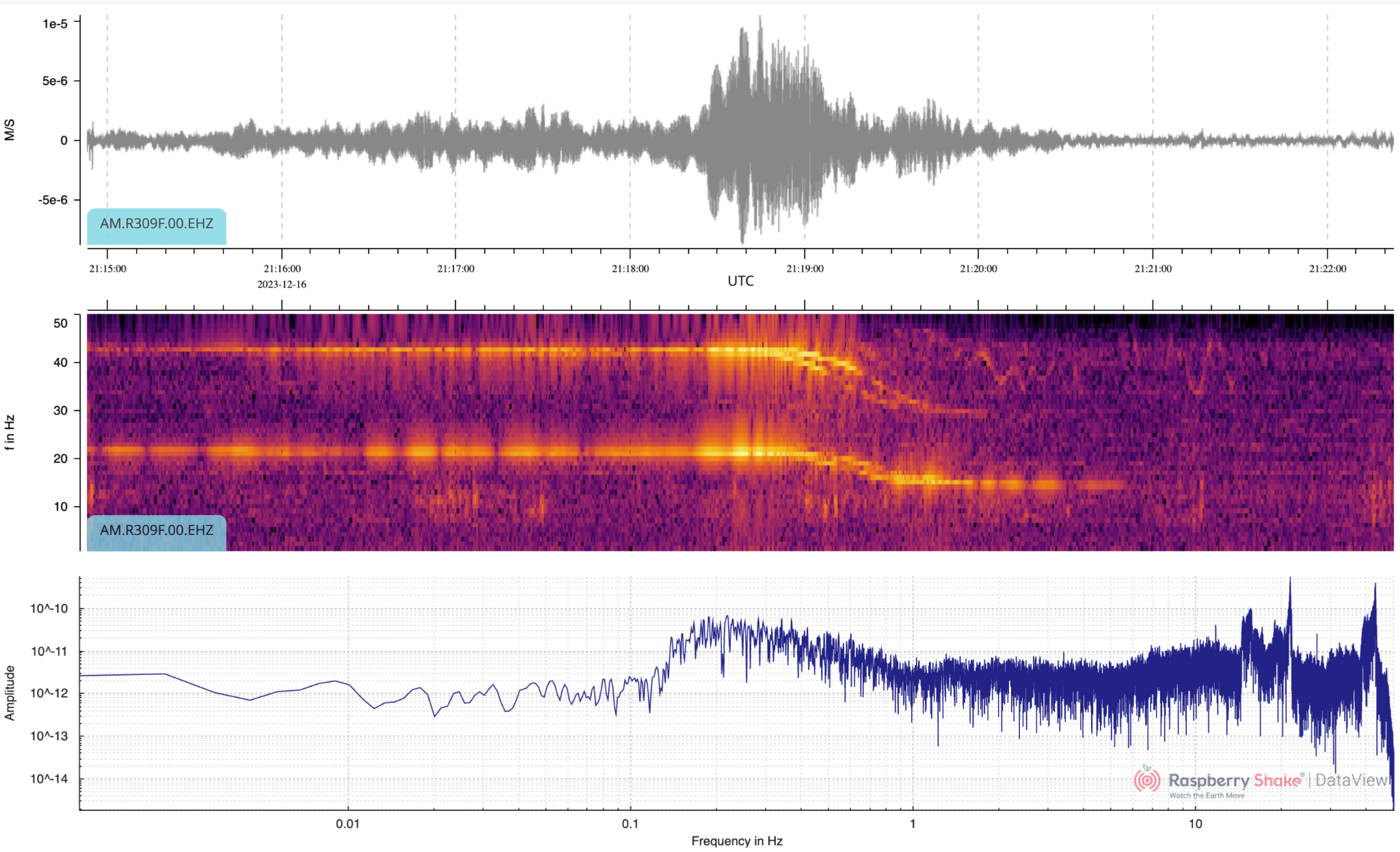
As shown in the top plot of Figure 2, helicopters often appear as a broad, relatively smooth signal that gradually increases and decreases in amplitude as the aircraft approaches the Shake location and then moves away.
But what really gives helicopters away is the spectrogram display (Figure 2 – central plot), with one or more solid lines that change frequency as the aircraft flies past (due to the Doppler effect). The number of traces varies, with larger multi-rotor helicopters having more.
The Doppler signature
Helicopter signals typically show one or more strong horizontal frequency lines that curve over time.
This is caused by the Doppler effect, in which frequencies shift as the helicopter first approaches and then moves away from the detection location. The effect is especially obvious when the helicopter passes close to the Shake or directly overhead.
As mentioned, larger helicopters may show several parallel lines in the spectrogram. These are harmonics produced by multiple rotor blades, engine components, and other rotating systems.
Because rotor systems generate continuous vibration, helicopter signals often appear much cleaner and more organized than the irregular broadband signals produced by vehicles or weather.
Estimating helicopter speed
As an interesting exercise, if the helicopter passes more or less overhead, you can use the information from the frequency display to calculate its speed.
Pick one of the lines and estimate its maximum and minimum speed from the graph as closely as you can. Using the upper trace in Figure 2:
The velocity is given by:
Where \(v\) is the speed of sound (767 mph, or 1234 km/h) and \(v_s\) is the speed of the helicopter.
The formula works by recognising that the fractional frequency shift equals the ratio of the helicopter’s speed to the speed of sound. Plugging in our values:
\[ \begin{aligned} v \cdot \frac{44 - 28}{44 + 28} &= v_s \\[6pt] v \cdot \frac{16}{72} &= v_s \\[6pt] 767 \text{ mph} \cdot 0.222 &= 170.4 \text{ mph} \quad (274.2 \text{ km/h}) \end{aligned} \]
This helicopter was travelling at approximately 170 mph. Fast, but well within the operating range of many military and coastguard helicopters.
So when a helicopter flies over your house, and everything rattles, it’s not your imagination. They really do shake the ground.
Seismic and infrasound detection
Here’s another example of a helicopter flying very close to Raspberry Shake and Boom station R5968 (Figure 3):
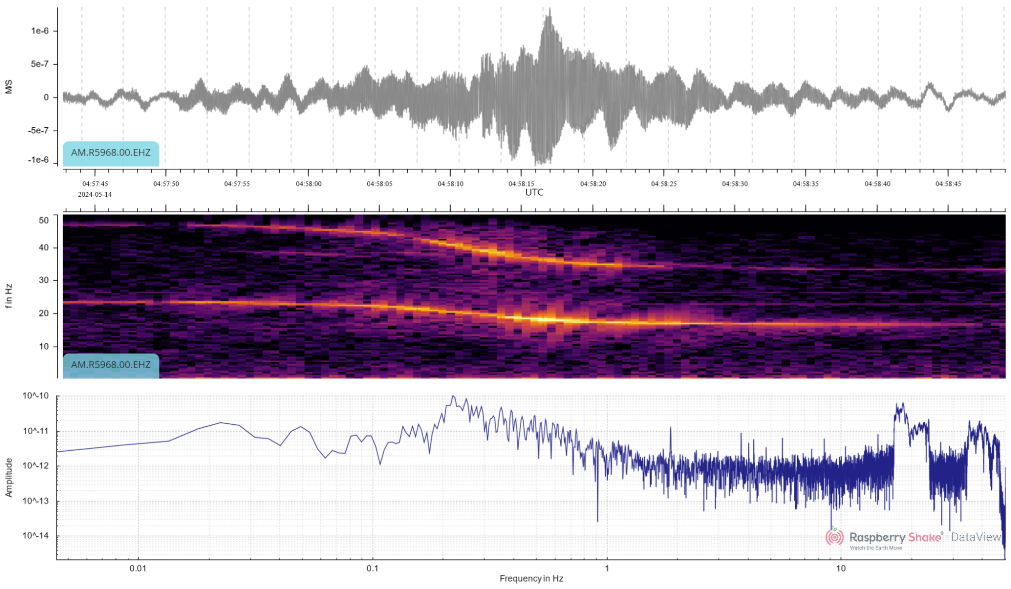
This is a strong signal on the EHZ channel, showing the typical Doppler effect. On this occasion, it was also strongly detected in the infrasound (HDF) channel (Figure 4):
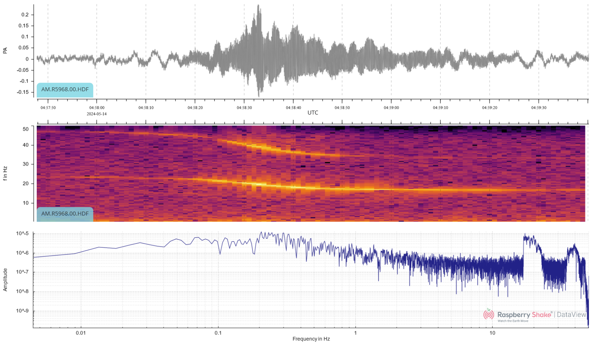
Figure 4: helicopter signal for station R5968 – HDF channel
Another example of a helicopter directly over Raspberry Shake and Boom station R21C0 (Figure 5):
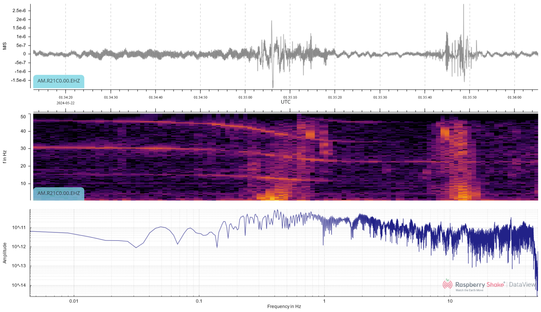
Figure 5: helicopter signal for station R21C0 – EHZ channel
Notice the different number of frequency lines (harmonics) in the Spectrogram. Again, easily detected on the EHZ channel (Figure 5) and the HDF channel (Figure 6):
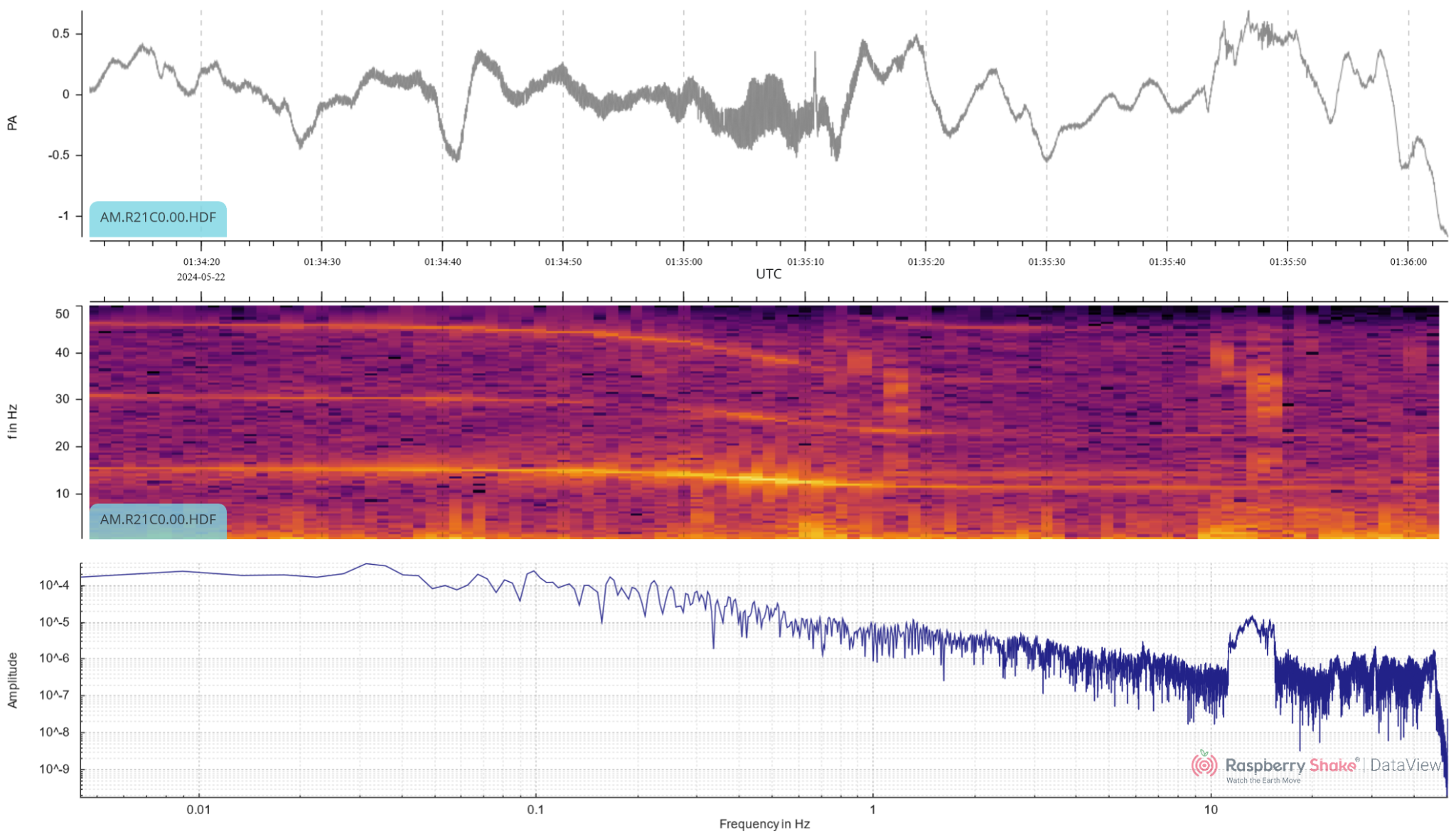
Figure 6: helicopter signal for station R21C0 – HDF channel
Below, instead, we have an example showing a low-altitude helicopter performing power line inspections with multiple turns (Figure 7). The Doppler shift reveals the frequencies of the signal rising and falling as the chopper approaches and recedes from the station, respectively. The intermittent signal at 30Hz is from vibrating rollers used on road works 300 to 1500 meters from the station.
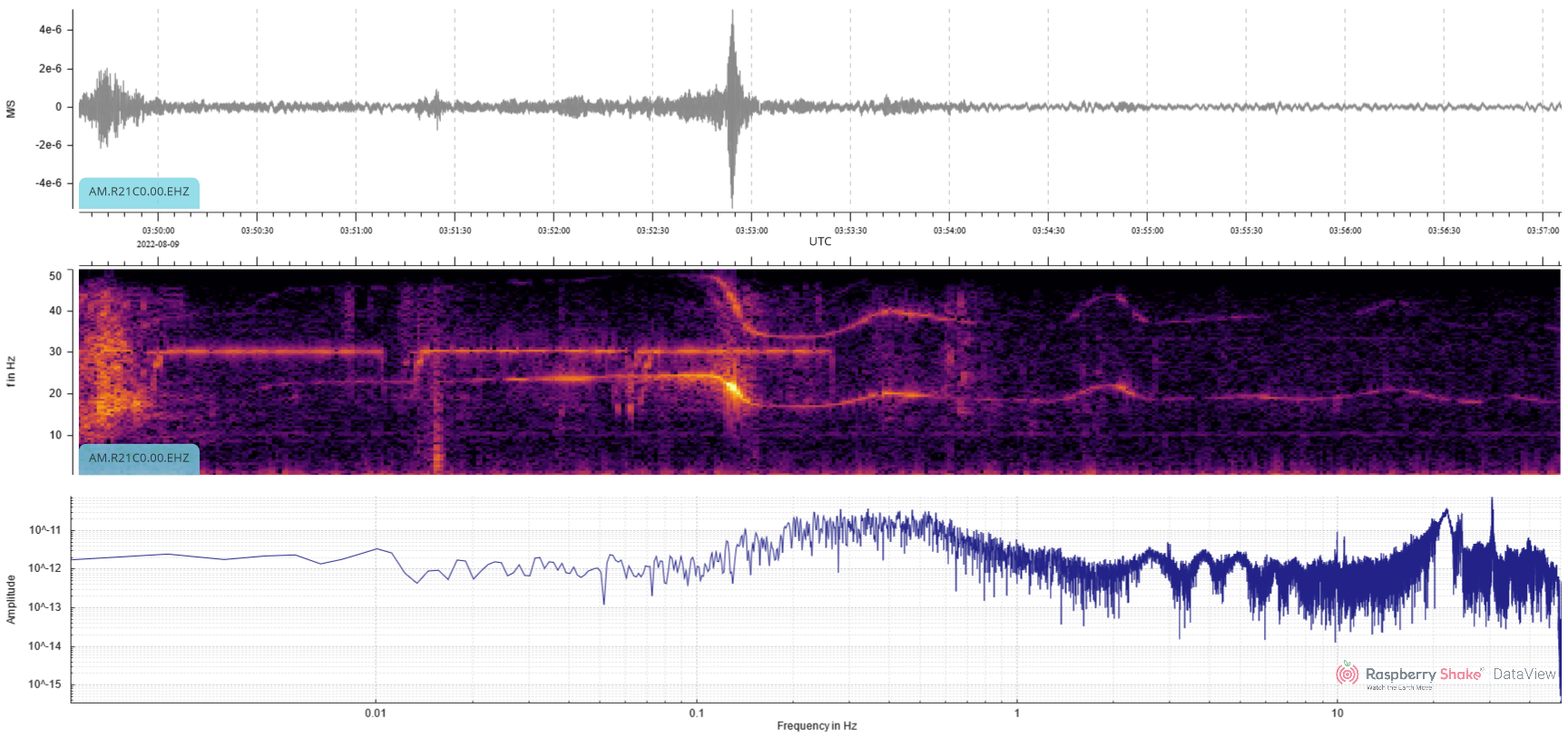
Figure 7: low-altitude helicopter over a prolonged period of time
Supersonic Fighter Jet
Most aircraft produce relatively smooth and continuous signals, but supersonic aircraft are different.
When an aircraft exceeds the speed of sound, it generates a shock wave that propagates outward through the atmosphere as a sonic boom. Unlike the rolling harmonic signature of a helicopter, a sonic boom appears as a sudden, impulsive event with a very distinctive waveform.
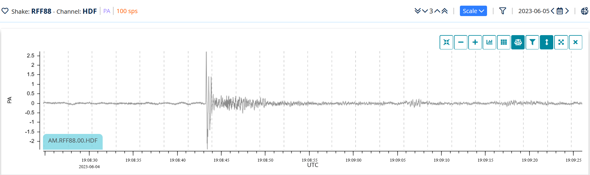
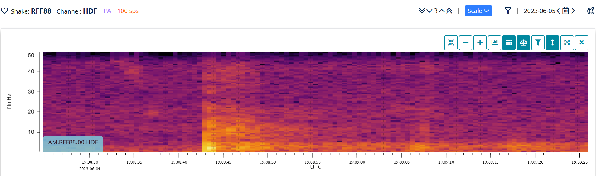
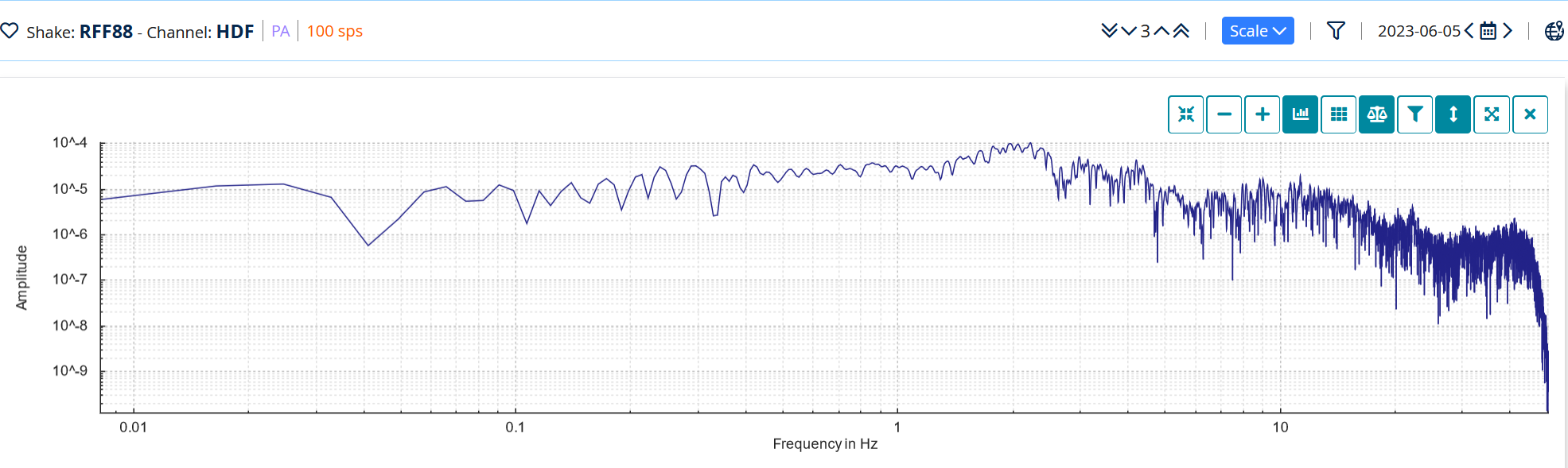
Figure 8 shows an example of a sonic boom from a US military fighter jet allowed to go supersonic over Washington, DC, to intercept an unresponsive plane (news article about this event).
The waveform shows a sharp positive spike consistent with a sonic boom. Immediately following is about 2.5 to 3 cycles at about 2Hz (measured by counting cycles on the waveform when zoomed in).
Following that, the signal decays to a significantly lower amplitude as the boom echoes from the surroundings and mixes with the sound of the jet engines. This matches the broad peak in the PSD plot at 2Hz (Figure 8 – bottom plot).
As a concluding note for this paragraph, remember that not every sonic boom is generated by a supersonic aircraft. As we will see in the coming paragraphs, meteors, spaceships’ re-entry, and more, can generate very similar signals. Expand your search for the source of the boom by checking local real-world information to confidently identify these events.
Spacecraft & Co.
Space Junk/Spacecraft Re-Entry
Some of the most unusual signals detected by Raspberry Shake stations originate far away from the depths of the Earth.
Rocket launches, re-entering spacecrafts, and falling space debris can all generate powerful atmospheric pressure waves that can travel enormous distances.
Depending on the event and the station configuration, these signals may appear:
- in the HDF infrasound channel
- on seismic channels through ground coupling
- or on both simultaneously
Unlike earthquakes, spacecraft-related events are usually dominated by acoustic shock waves traveling through the atmosphere rather than seismic energy propagating through the inside of the planet.
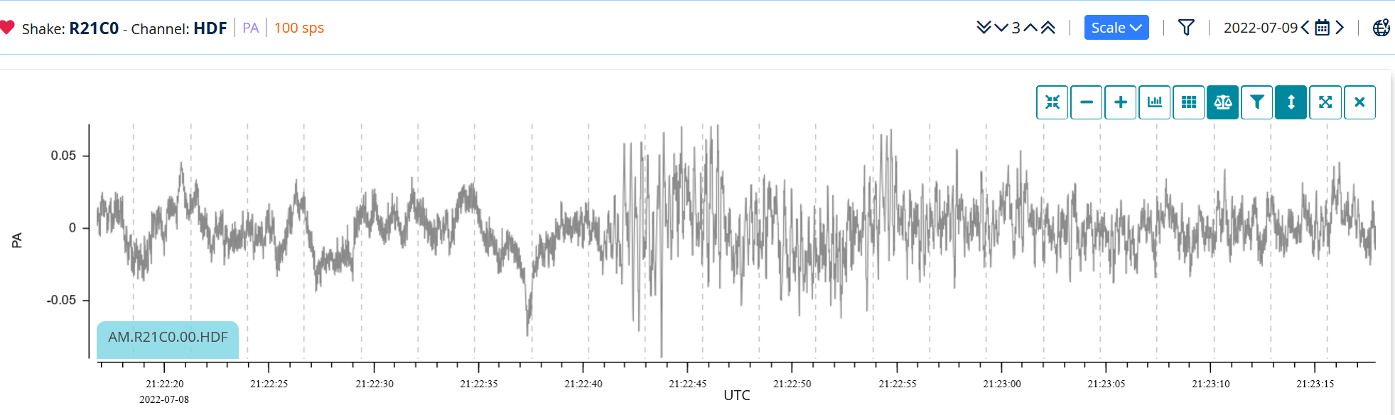
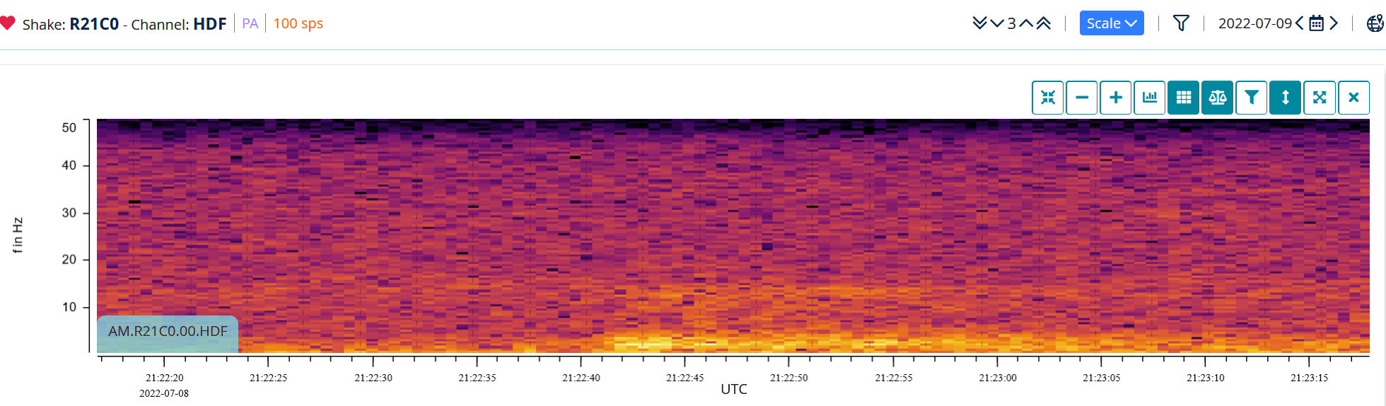
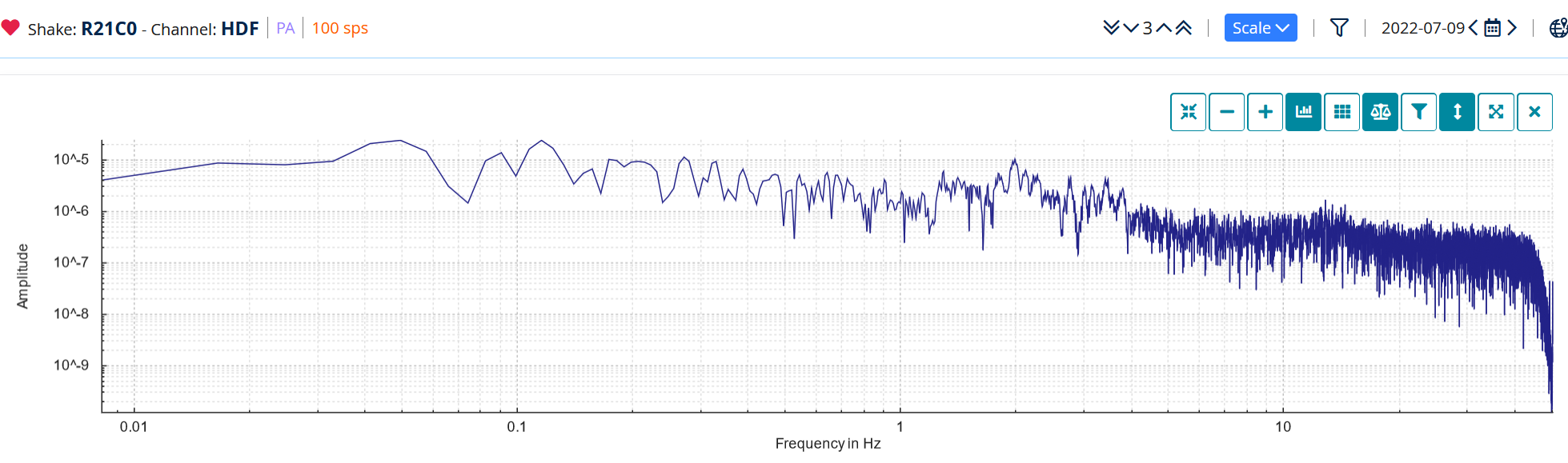
This example from 2022 (Figure 9) shows the SpaceX Crew-1 Dragon trunk reentering the atmosphere over Victoria, Australia, at 21:05 UTC.
The re-entry path was 370 km from the station at its closest approach, hence the signal arrival at around 21:23 UTC. The signal is very strong below 4 Hz and is typical of a continuous sonic boom made by space junk re-entering at a distance. This time, the signal was not detectable on the EHZ channel of the Raspberry Shake and Boom.
Rocket Launches
Rocket launches produce a different kind of signal from the just-seen re-entry waveforms.
Instead of a fast-moving shock wave crossing the atmosphere, launches generate sustained acoustic and ground vibration from the rocket engines themselves.
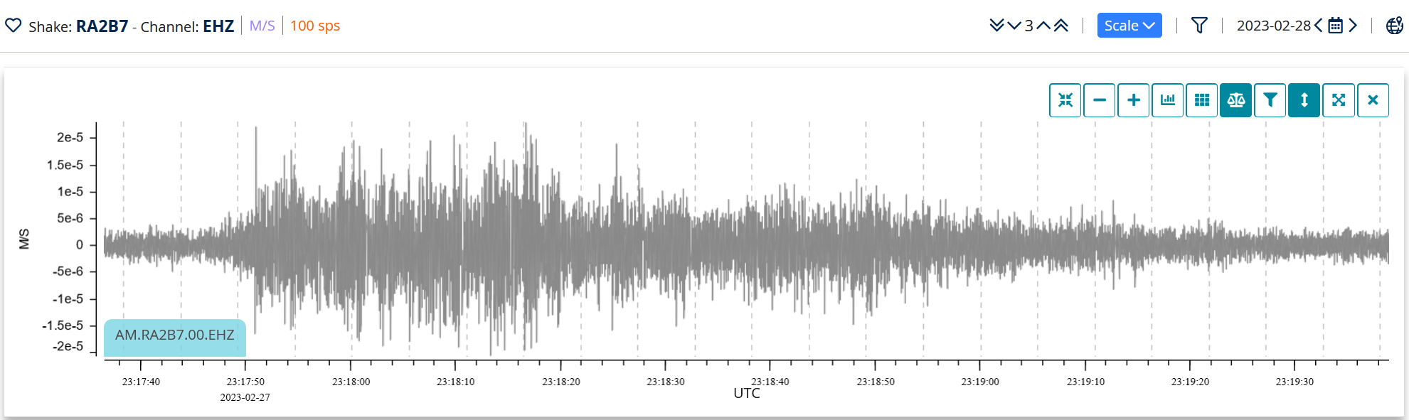
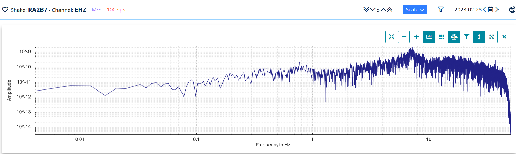
This example (Figure 10) is the acoustic arrival of a Falcon 9 Starlink Rocket Launch detected on the EHZ channel of a 3D Shake. The rocket acoustic signal arrives at 23:17:50 UTC. The PSD shows a peak at 7 Hz, and a very strong broadband signal above 0.3 Hz.
Luckily, compared to aircraft sonic booms, re-entry and launch windows are usually planned well in advance. So, if you live near a re-entry corridor or near a spaceport, you can easily cross-reference the waveforms your Shake has captured and discover which space-related event was recorded!
Spikes
Not every unusual-looking signal comes from inside the Earth, or even from the outside world. Spikes broadly fall into a few categories: those with an identifiable source, those of uncertain local origin, and those due to periodic interference from electrical equipment. The examples below illustrate each.
These signals are important to understand because they can easily be mistaken for meaningful seismic events, especially when they produce large spikes or unusual patterns.
Spikes occur from time to time. For some, it’s easy to determine their source. Instead, and at length, others have been discussed in the discussion group without reaching any accurate conclusion about their source.
The helicorder snapshot below (Figure 11) shows two spikes:
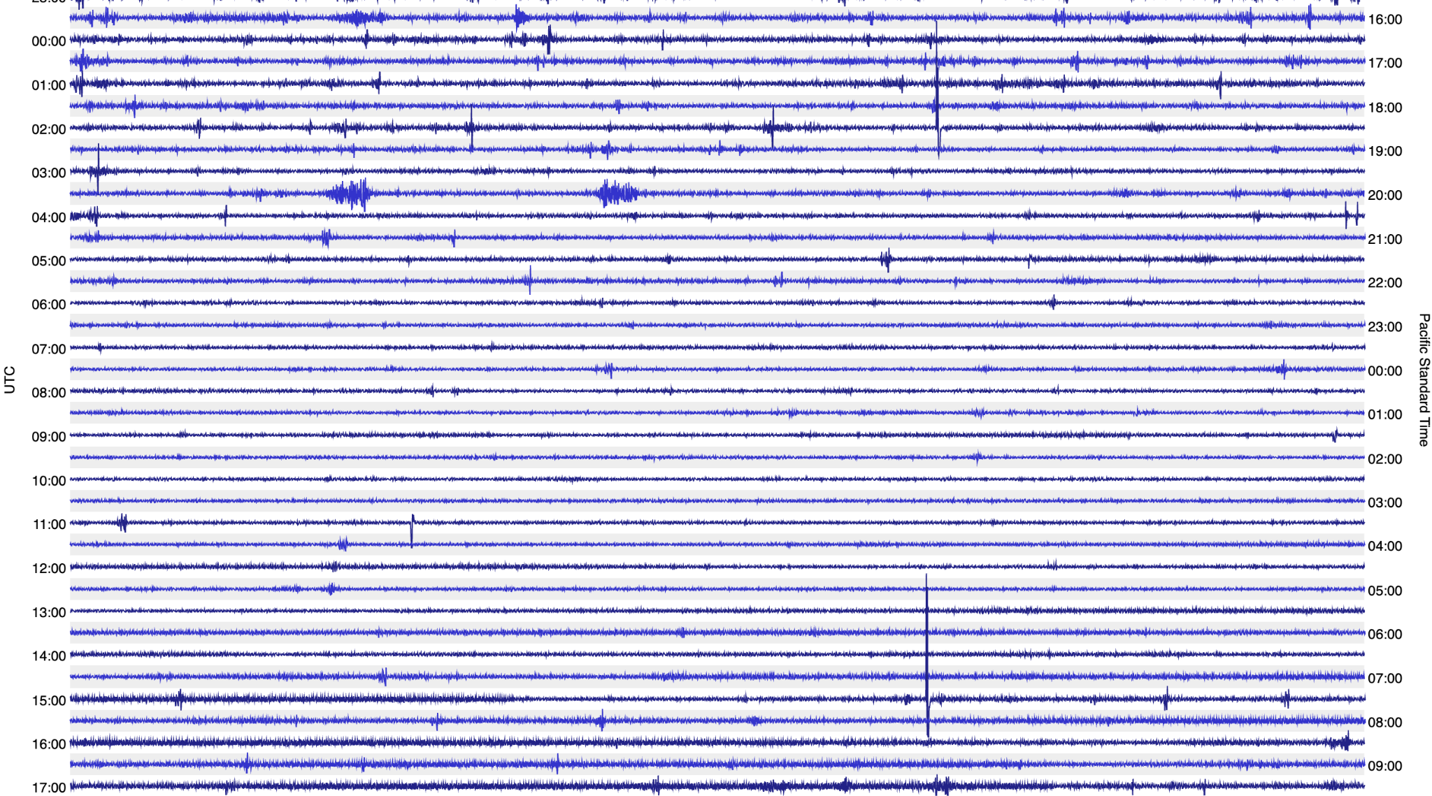
The upper one looks like this when expanded (Figure 12):
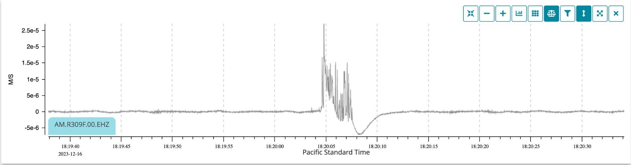
In this case, the source was straightforward: an Amateur Radio transmitter (used by author) operating at approximately 1 kW at 3.96 MHz. It’s difficult to shield any electrical device against that sort of RF field.
The lower spike is one of those of indeterminate origin (Figure 13):
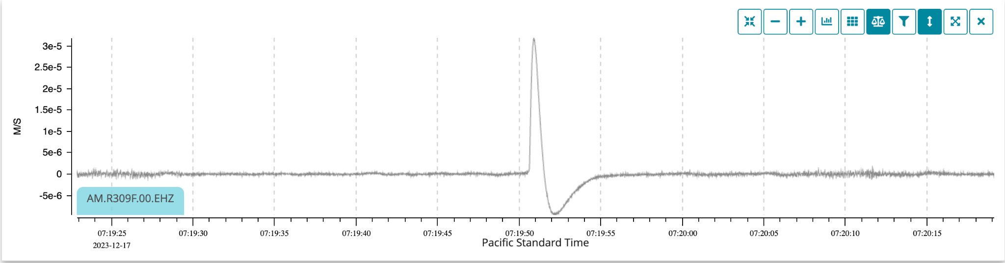
These always have the same form, a very large positive (or negative) spike with a small overshoot as it returns to the “zero” line. They occur randomly.
One plausible explanation is the placement of the Shake on a large concrete slab: in this case, the floor of a pole barn. Temperature changes can cause stresses in the slab that release suddenly as a sharp crack, and the same can happen with metal walls or a roof.
Notably, nearby Shakes did not detect these spikes, confirming that whatever the source, it is extremely local.
Then there are these (Figure 14):
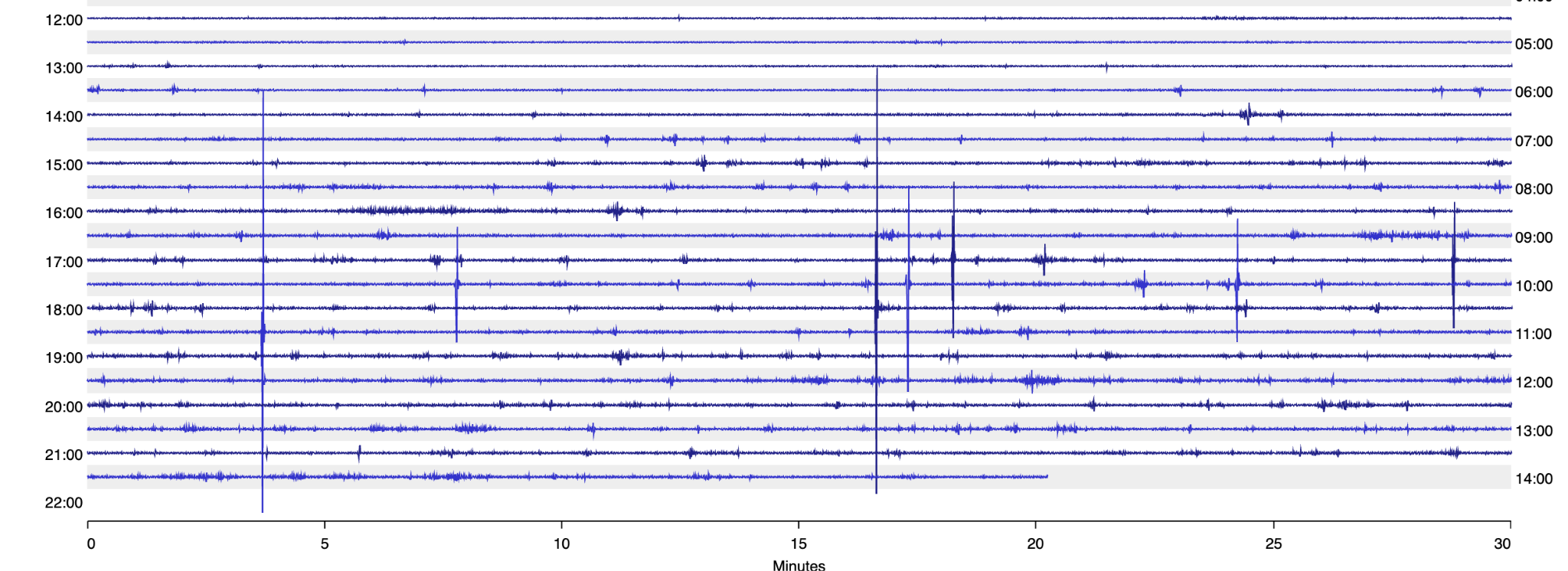
They are not the same. If we examine the big one on the furthest left (Figure 15):
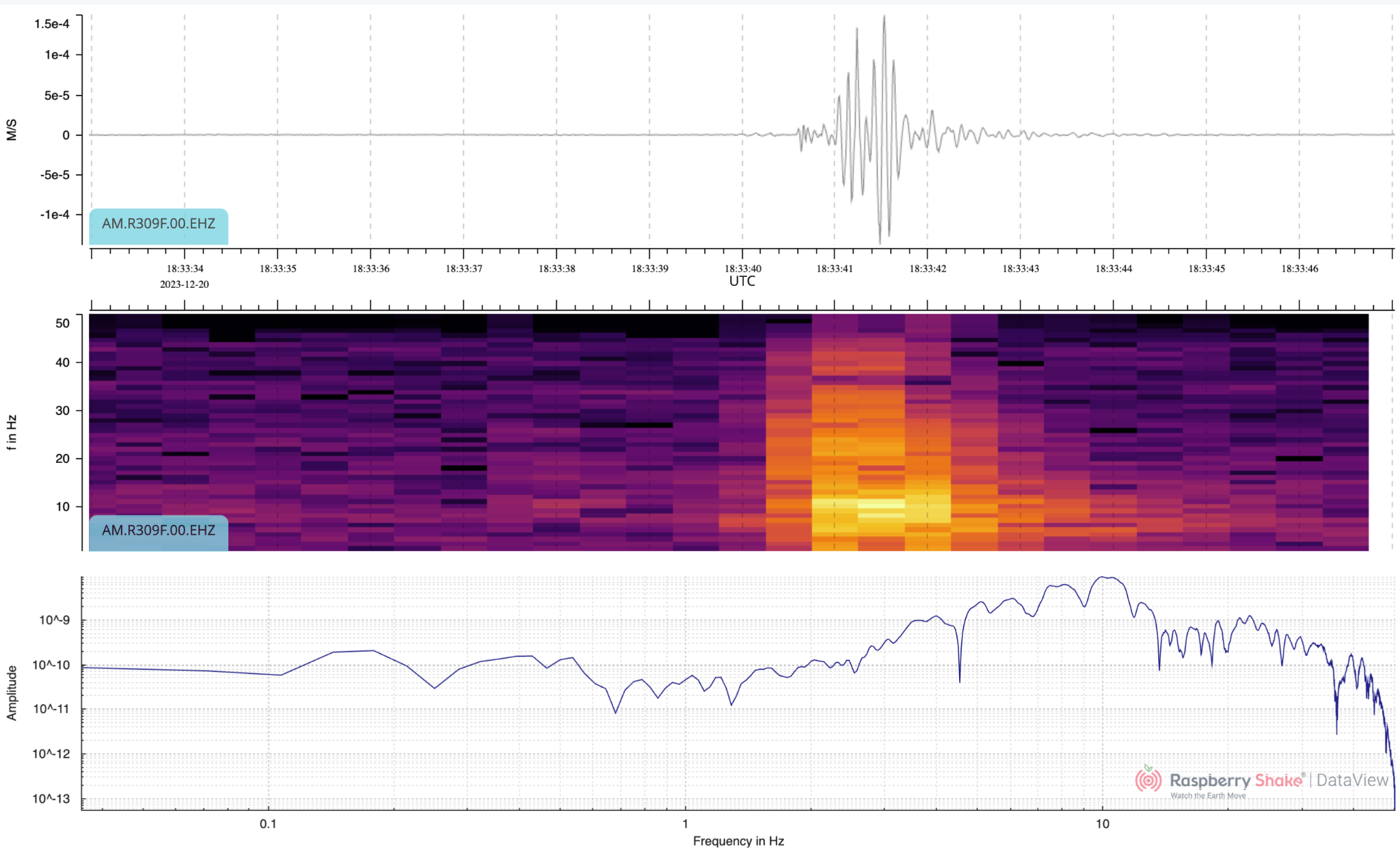
It oscillates at about 10 Hz. Around the time this was recorded, some work was going on trimming and cutting down trees not far away. Related? It is hard to know unless you are carefully watching as the tree work progresses and see when trees/branches fall, and if a corresponding event is recorded on the seismometer.
Electrical Interference
The following example is from a Raspberry Shake and Boom when a Power Over Ethernet (POE) power supply was trialed. Unfortunately, this specific POE supply induced unacceptable interference with the vertical EHZ channel. (Note there are POE supplies that have suitable filtering, so this doesn’t happen). No interference was evident on the HDF channel (Figure 16):
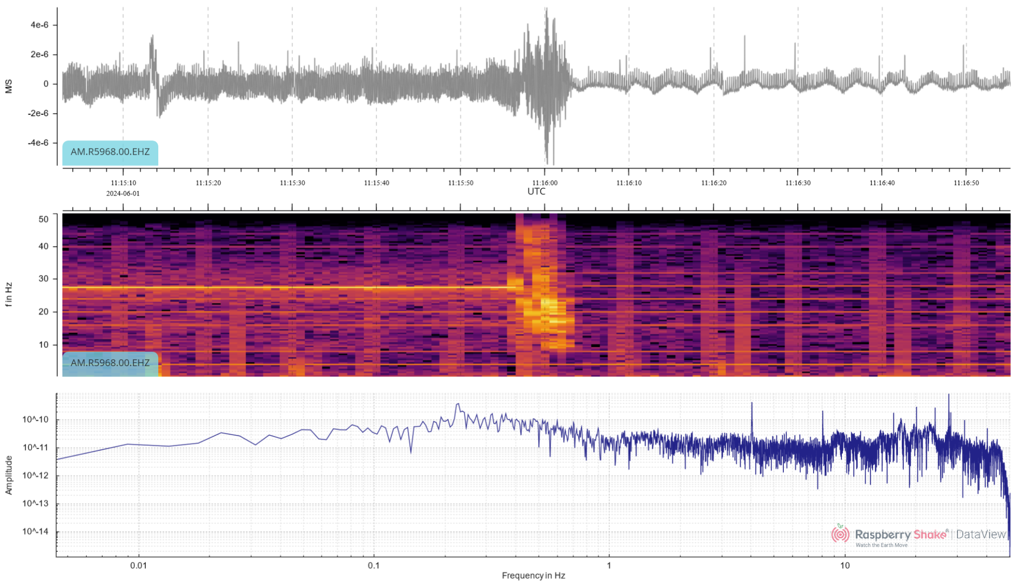
The electrical interference is visible in the right-hand half of the waveform. The left half of the waveform is dominated by the seismic signal of a water pump 5 meters away on a separate concrete plinth.
In the spectrogram, the electrical interference is shown as many horizontal lines, which are harmonics of the frequency of the small spikes seen in the waveform: 4 Hz – so there is a small spike every 0.25 s. Vertical lines appear whenever a larger spike appears in the waveform. Interestingly, the 3x harmonic (12 Hz) is missing.
The PSD shows the frequencies of the harmonics of the interference as well as the frequency from the water pump: 27.5 Hz – very close to the 28 Hz spike from the interference. The 27.5 Hz of the water pump corresponds to a pump shaft speed of 1650 rpm, which is quite unusual for either 50Hz or 60Hz systems. This installation is off-grid.
Explosions
Explosions are among the most dramatic signals a Raspberry Shake can detect, but not all of them look the same. Some occur in the atmosphere while others originate underground. We will use the following list to broadly categorize them:
- Atmospheric explosions
a. Lightning
b. Meteors, Fireballs, and Bolides - Mine or Quarry Blasts
- Explosions associated with volcanic eruptions
- Underground Nuclear Tests
Atmospheric Explosions
Atmospheric explosions produce a pressure wave in the atmosphere, which may be detected directly by a Raspberry Boom or Raspberry Shake and Boom in the infrasound HDF channel. They can be artificial or natural, such as lightning or sonic booms from meteors, bolides, or space junk re-entry.
The atmospheric wave may also interact with the ground to become a seismic P wave, making it detectable on any Shake.
Let’s start with two of the most common natural atmospheric events: lightning and meteors.
Lightning
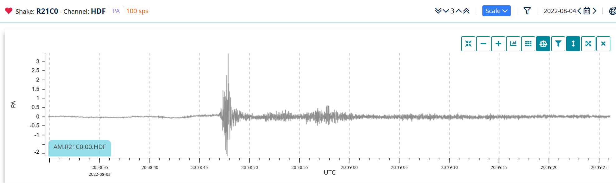
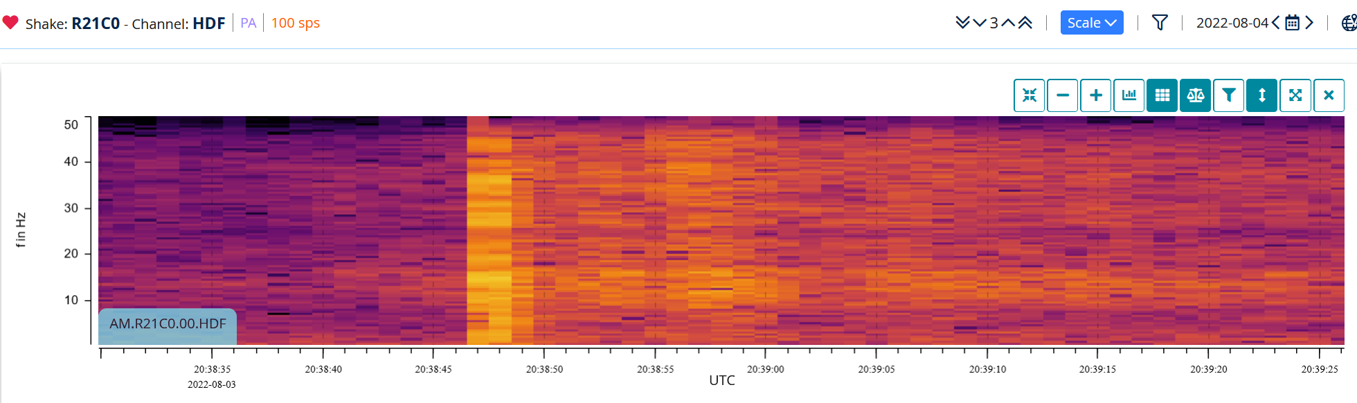
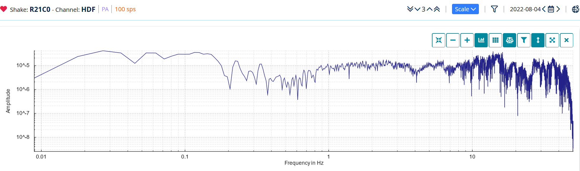
Below are the Waveform, Spectrogram, and PSD for a particularly loud (and close) lightning strike detected in infrasound on Raspberry Shake and Boom R21C0 (Figure 17):
Compare these to the EHZ (vertical seismic) channel (Figure 18):
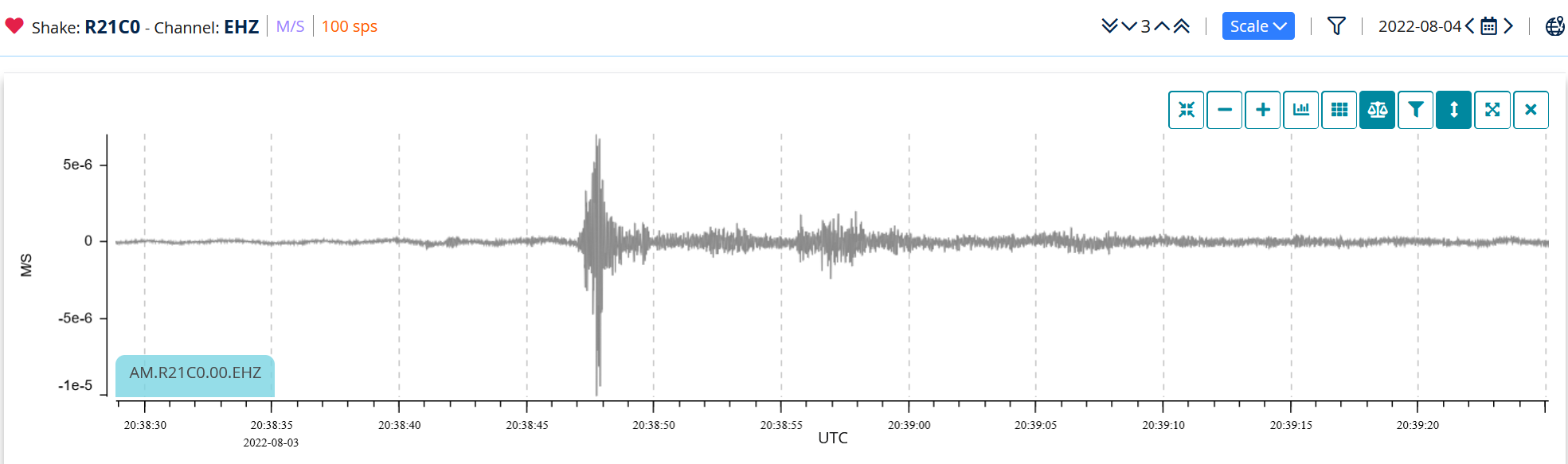
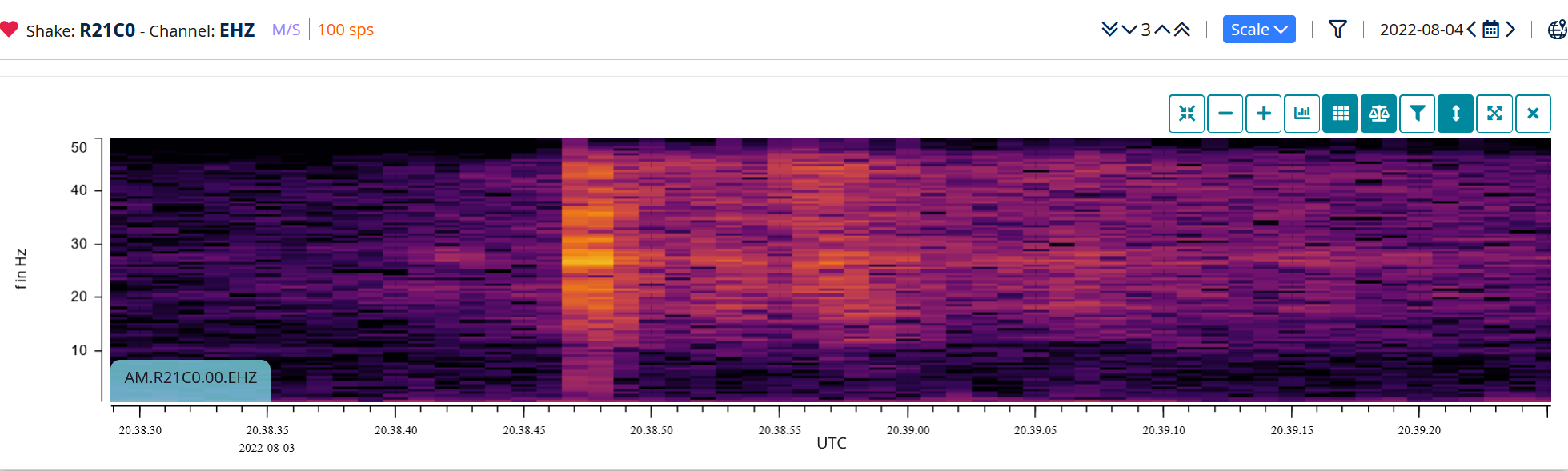
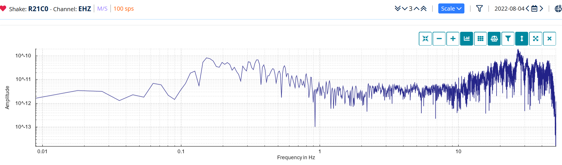
Notice the waveforms look pretty similar between the HDF and EHZ channels, so detection of close atmospheric explosions is feasible with a simple Shake, but also notice that the PSD and Spectrograms show a lack of coupling between the atmosphere and the ground below about 10 Hz: i.e., the EHZ signal is weak below 10 Hz.
Also note that, since the lightning strike was close, high frequencies have not yet been attenuated. Explosions and lightning strikes farther away will likely show reduced intensity at higher frequencies due to attenuation.
Meteors, Fireballs and Bolides
Meteors (also known as shooting stars) are small meteoroids about the size of a grain of sand up to about the size of a pea that burn up when entering the Earth’s atmosphere. As they enter the atmosphere between 11 km/s and 73 km/s, they are well beyond the speed of sound (0.34 km/s), so a sonic boom is produced as they pass through the air. Fireballs and Bolides are larger examples that may not completely burn up in the atmosphere.
The sonic booms from meteors, fireballs and bolides are detectable directly in infrasound using a Raspberry Boom (or a Shake and Boom) and indirectly by a Raspberry Shake when the pressure wave is big enough to excite the ground. An example is shown in Figure 19 below, where we can see the brief, broadband nature of the signal in the spectrogram and the sharp impulse in the waveform. Quite different from the other signals we have seen so far.
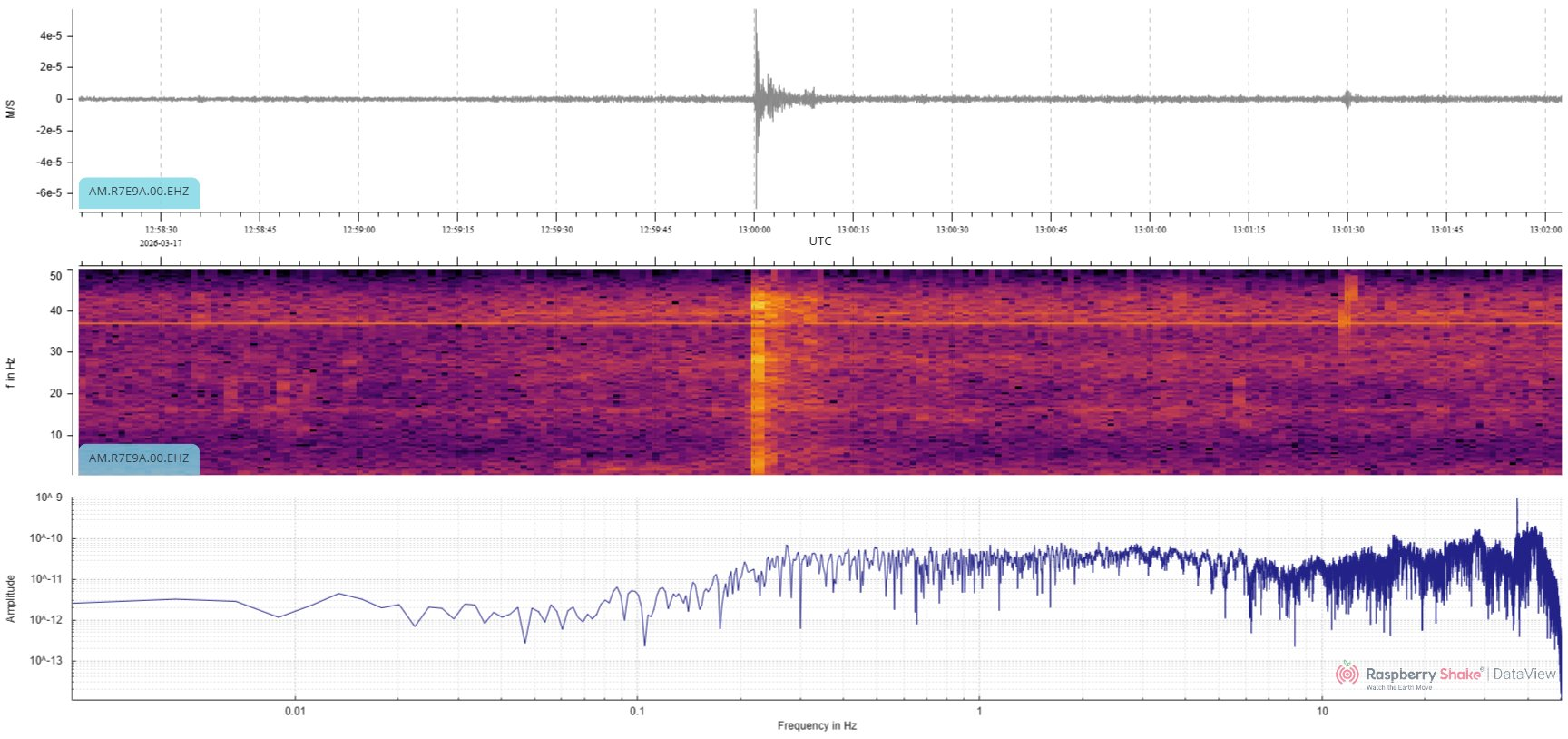
What does a meteor detection actually look like on your Shake, and how do you distinguish it from other impulsive events like lightning or a nearby explosion?
The waveform characteristics to look for are:
The signal is typically brief and impulsive, much shorter in duration than a quarry blast or volcanic event, and without the sustained coda you’d expect from an earthquake. On the EHZ channel, it appears as a sharp spike followed by a relatively rapid return to background noise.
On the spectrogram, the energy is broadband, covering a wide frequency range simultaneously, similar to a lightning strike. Unlike a helicopter, however, there are no organised frequency lines or Doppler shifts.
Detection on the HDF infrasound channel is more reliable for smaller events, since the pressure wave from the sonic boom travels directly through the atmosphere to the sensor. The EHZ channel will only show a response if the pressure wave is strong enough to couple into the ground. This tends to require a larger fireball or a relatively close approach.
A practical recommendation for suspected recorded meteors: such events are logged by dedicated fireball networks (such as the American Meteor Society or the UK Meteor Observation Network), and major events are often reported within hours (or even minutes via social media). Cross-referencing your Shake’s timestamp with these databases is usually the quickest way to confirm a suspected detection, and a very satisfying one when it matches.
Mine or Quarry Blasts
Mine or quarry blasts can also include smaller blasts used in construction or road building, but generally, mine and quarry blasts are the larger examples.
Mine or quarry blasts are very similar to earthquakes in their signature but are generally limited to magnitudes less than about MLx 3.5.
As they are not really big, in seismic terms, most mine and quarry blasts will appear like a close small earthquake, as you can see on the following helicorder from a shake near Mudgee, NSW, Australia (close to the Ulan and Hunter Valley Coal Mining areas). The six circled events (Figure 20) are all mine blasts, showing the classic close earthquake signature of a P wave followed closely by the S wave.
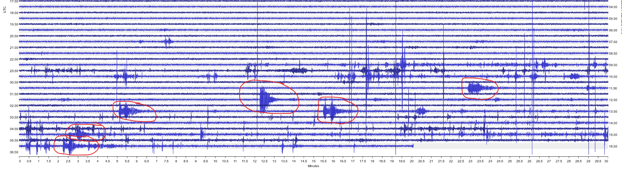
As with an earthquake, the time between the P- and S-wave arrivals indicates how far away the blast is. The P and S waves arrivals are very close on the second event on the helicorder, suggesting it is from a mine close to the station (probably the Ulan area), while the others are further afield (probably from the Hunter Valley).
The signature for a mine or quarry blast is exactly the same as for a small nearby earthquake. They are usually detected by examining the helicorder as above, then checking against nearby shakes. Typically, mine and quarry blasts are NOT REPORTED as earthquakes, so if you detect a possible small earthquake that isn’t reported officially, it may well be a small earthquake that hasn’t been detected on enough seismographs to be properly resolved, or it may just be a mine or quarry blast.
Occasionally, a mine blast will be detected like this one (Figure 21):
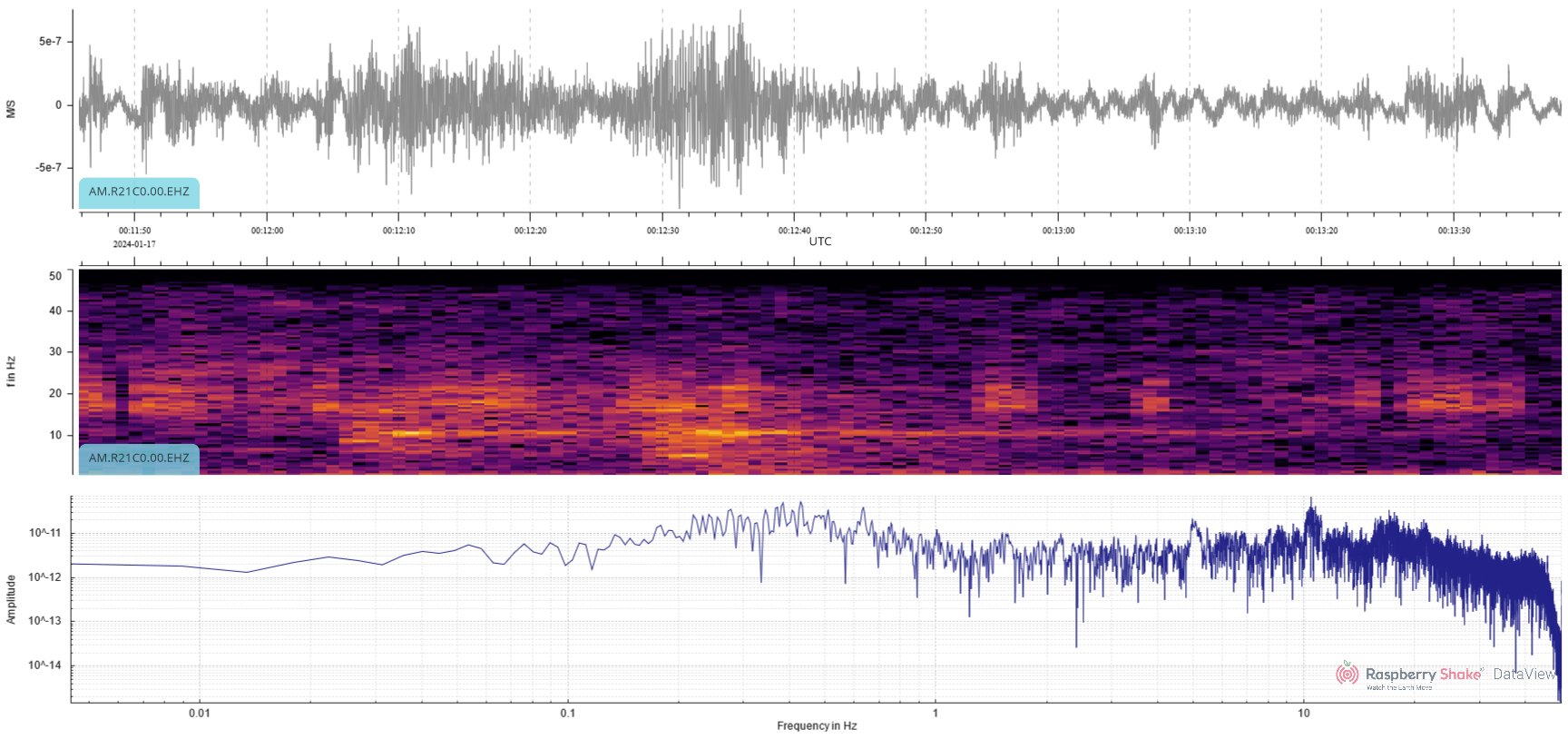
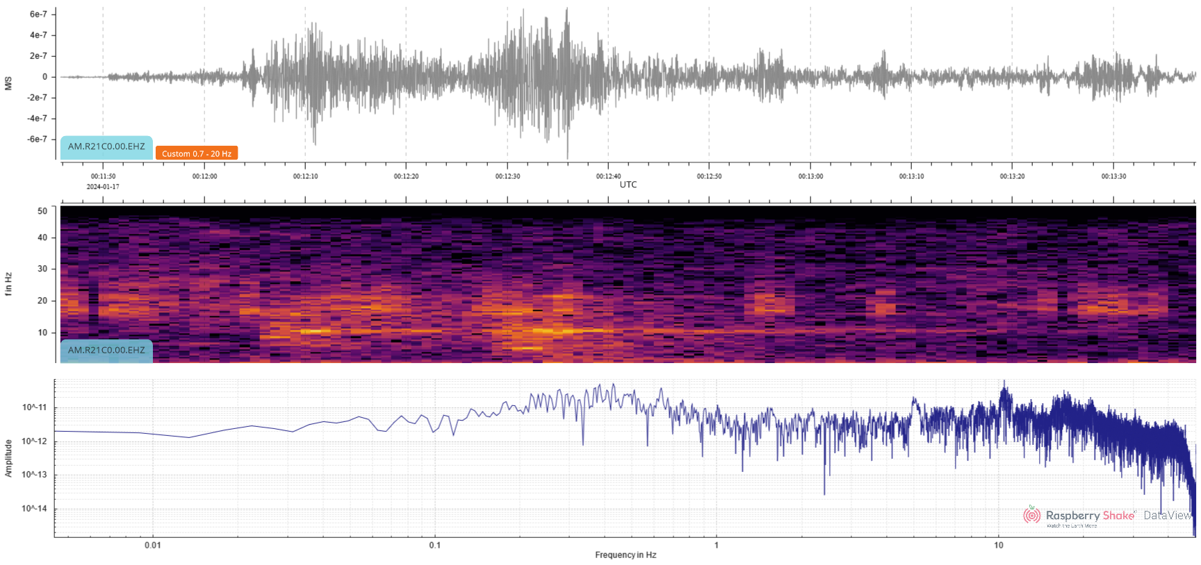
The P wave arrives at 00:12:04 UTC, and the S wave arrives at 00:12:28 UTC. Notice the line in the spectrogram at about 11Hz, which coincides with both the P and S wave arrivals (actually about 3 to 4 seconds late). This is a detection of the blast interval: 11 Hz yields a blast interval of 1/11 = 0.091 seconds between charges. Often, the detonation interval is more random, so a distinct line doesn’t show up, however.
The waveform is clearer when a filter is applied. In Figure 22, a 0.7 Hz to 20 Hz filter is applied to the same signal. The arrival of the P and S waves is much clearer in the waveform when an appropriate filter is applied.
Sometimes, a mine blast signal can look a little unusual because it may be very weak at frequencies below about 10 Hz, as shown in Figure 23.
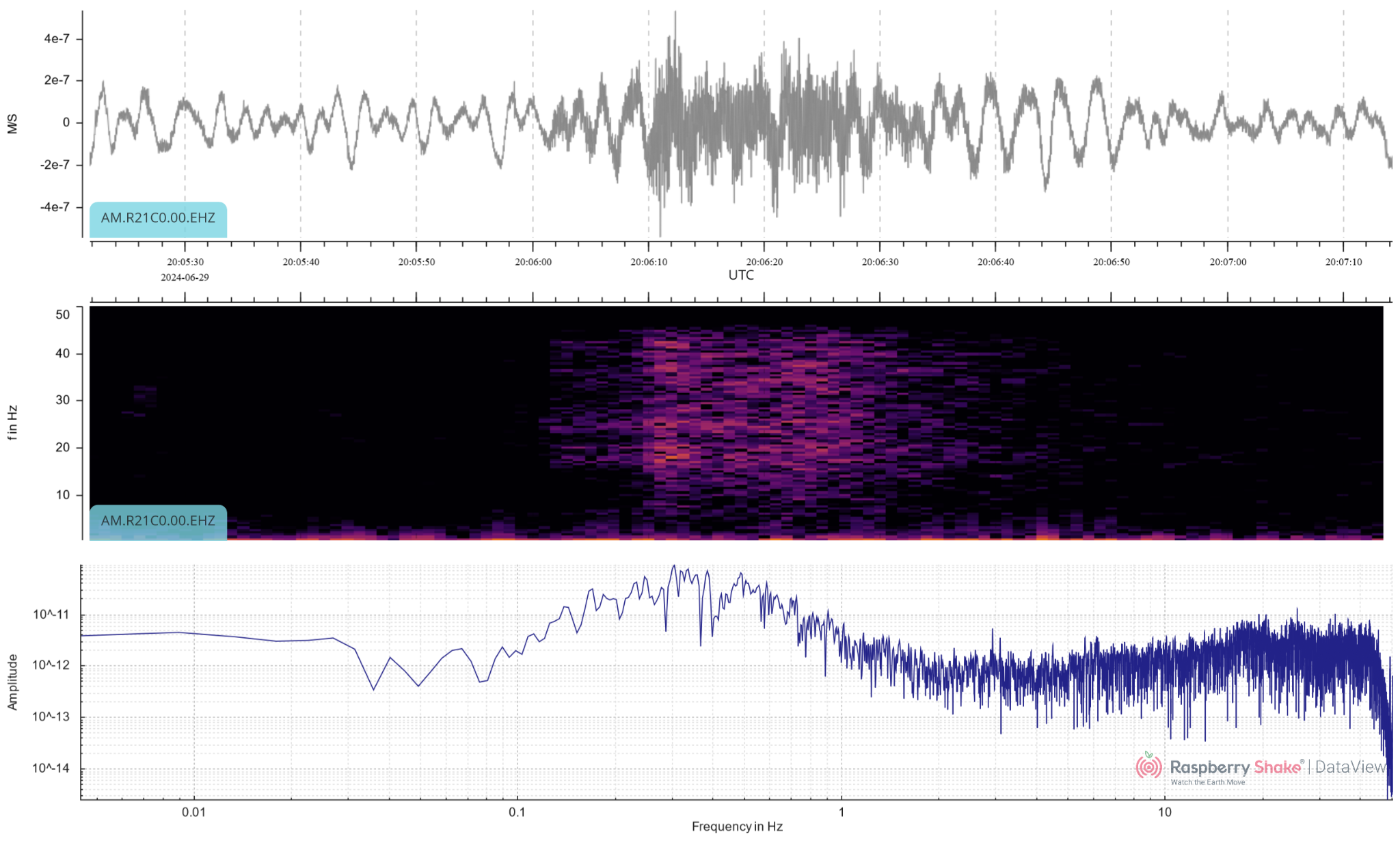
Notice, in this example of an M1.4 mine blast from a gold mine 80 kms away, the lack of or weakness of frequencies in the spectrogram around 10Hz. That’s clearly not an earthquake, yet there are P and S arrivals at about 20:06:10 UTC and 20:06:21 UTC, respectively.
Notice also that in this case, a signal from the blasting sequence is evident before the P arrival – starting at about 20:06:01 UTC.
These characteristics are not always visible in mine blast signatures, but when they do appear, they can distinguish a blast from an earthquake.
Explosions associated with Volcanic Eruptions
On January 15, 2022, the eruption of the Hunga Tonga-Hunga Haʻapai submarine volcano in Tonga resulted in atmospheric pressure waves that circled the world at least twice. Figure 24 shows the primary wave as received at Coonabarabran in New South Wales, Australia (about 3,700 km away).
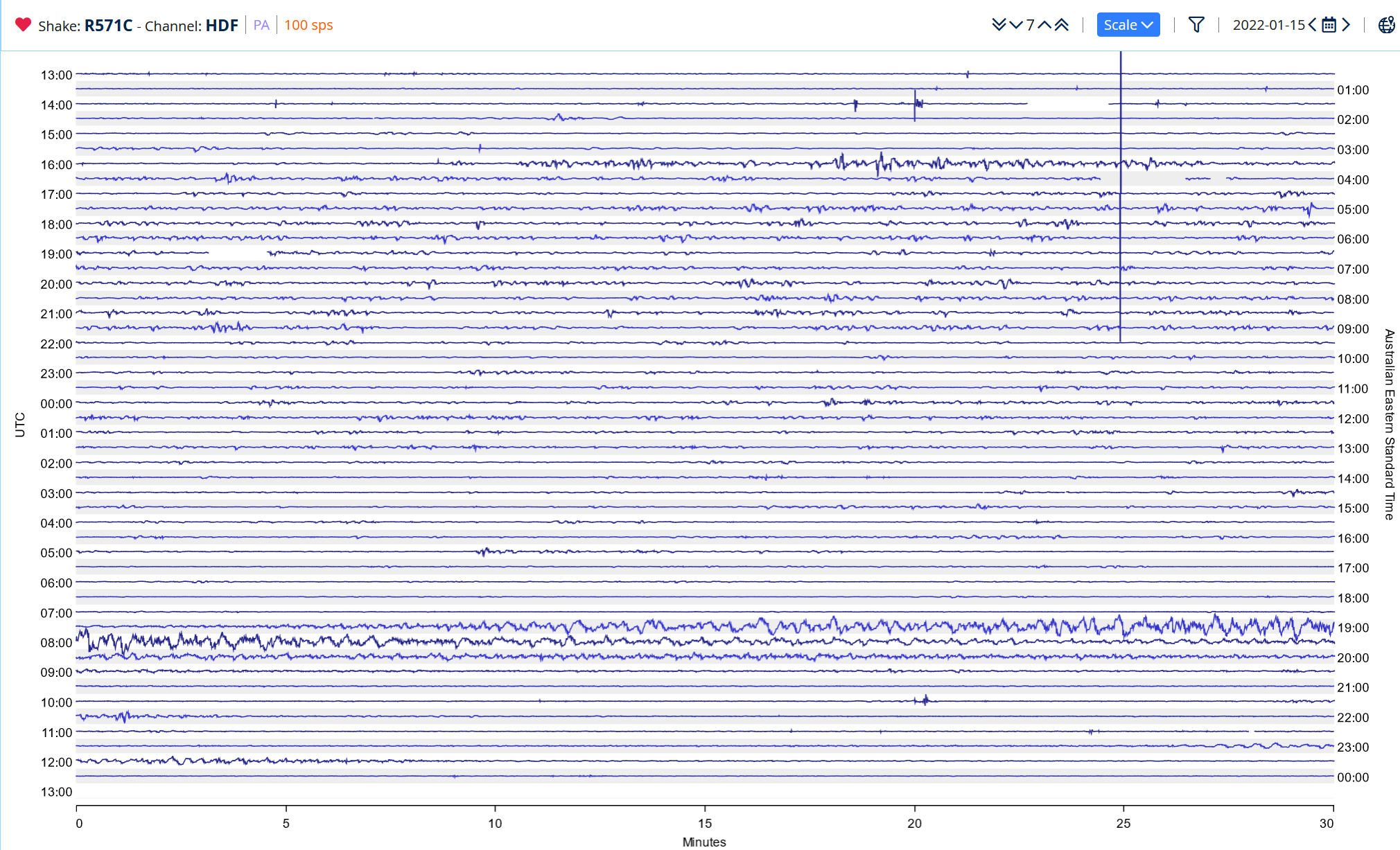
The infrasound begins arriving at 07:05 UTC and finally decays at about 09:05 UTC. Obviously, the explosion was not a simple, discrete boom, but continued for some time as gases were released.
Sampling the strongest 30 minutes of the signal with Dataview produces the plot in Figure 25:
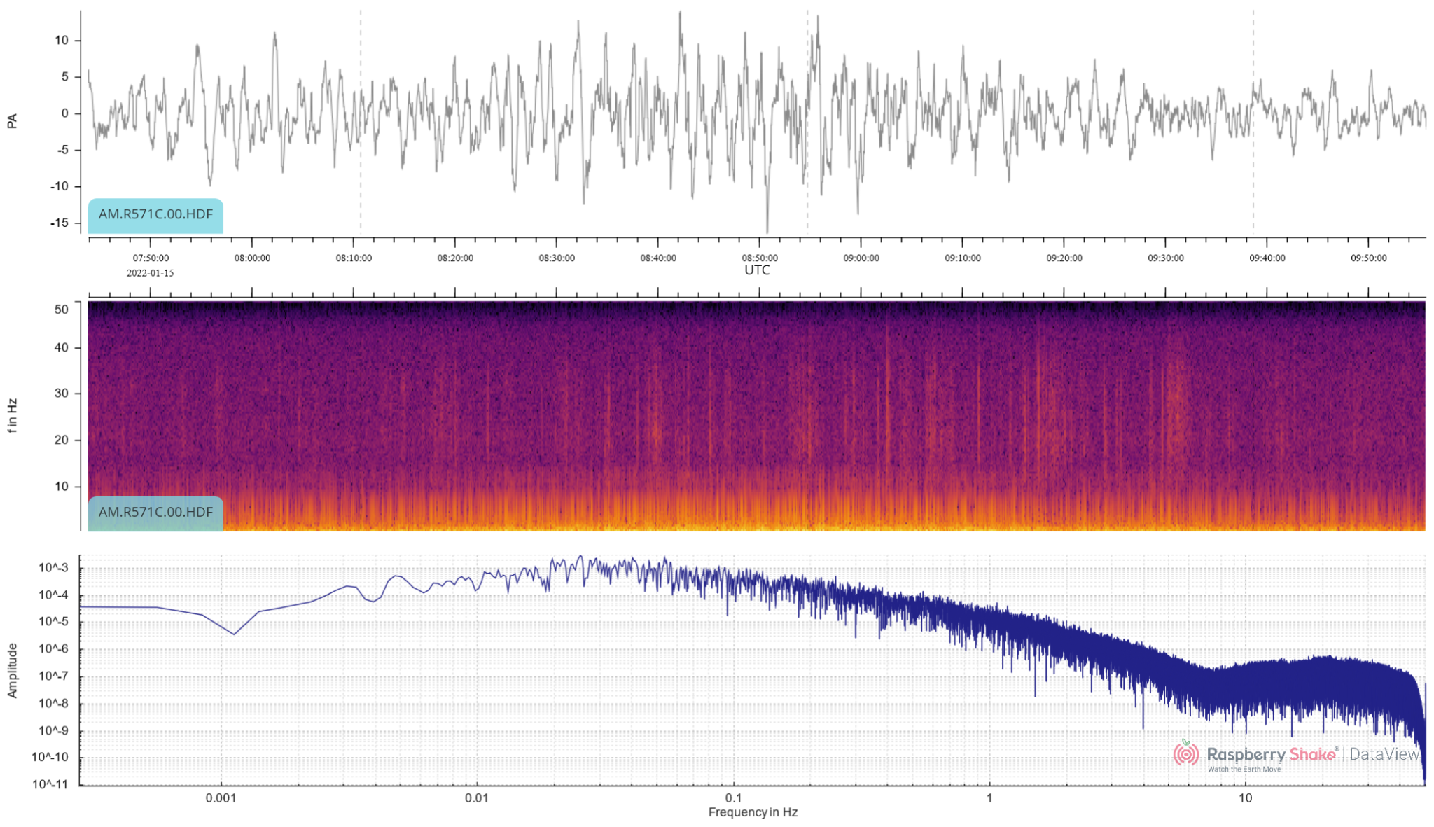
Notice the amplitude of the waveform – 15 Pa! That’s a pretty strong infrasound signal from 3700 km away!
The spectrogram is strongest below 15 Hz.
The PSD plot has a strikingly smooth curved appearance with a dip at 7 Hz. Clearly, a very strong broadband signal that overwhelms the background noise.
The same event from a slightly closer Raspberry Boom (R2DDD) in Christchurch, New Zealand (2700 km away) provides the following (Figure 26):
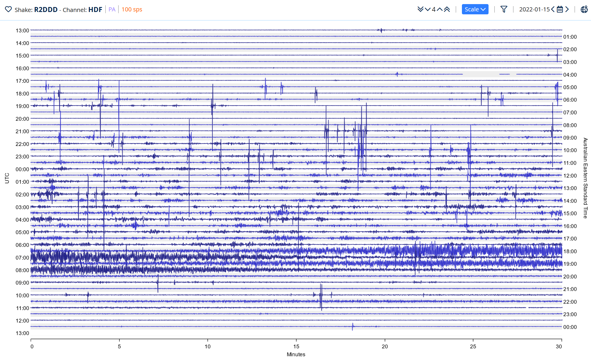
Interestingly, the helicorder shows the infrasound signal intensity building from about 8:40 UTC, then decaying by about 7:15 UTC, before building again at about 7:40 UTC and finally decaying at about 8:20 UTC. The fainter long-duration signal between about 10:30 UTC and 11:00 UTC is likely to be the combined signal from the wave going the long way round and the direct wave on its second time around the world. (40,000 kms x .33 km/s = 13200 s = 220 min = 3 hours 40 minutes).
Again, selecting the strongest 30-minute sample in Dataview gives the plot in Figure 27:
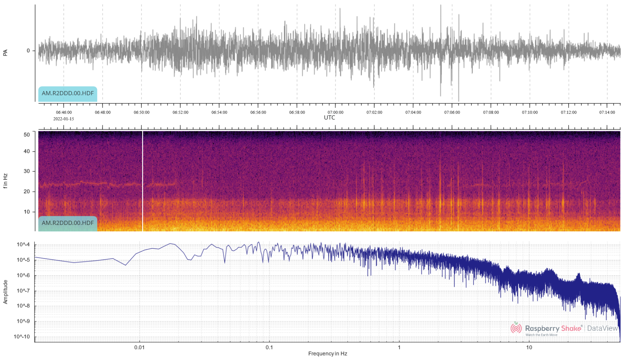
The signal contains more noise than the previous example from R571C, so the overall amplitude is not a good comparison without some filtering.
The spectrogram shows a stronger signal, as expected, being closer to the source. There are also higher frequencies, which are evident up to about 17-18 Hz.
The PSD again shows a strong broadband frequency curve, with some noise influence above about 18 Hz.
Underground Nuclear Tests
Underground Nuclear Tests are fortunately rare but are unique in their signature. The whole idea of the underground nuclear test is to fully contain the explosion and measure its power by seismically measuring the P wave produced. As the surrounding rock fully contains the blast, there is little to no shearing of rock during the blast, so there is no appreciable S wave.
So, the signature for an Underground Nuclear Test is a P wave with no following S wave.
Two of the earliest deployed Raspberry Shakes in South Korea managed to capture the September, 3, 2017, North Korea underground nuclear test, shown in Figure 28:
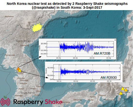
It’s worth noting that detecting exactly this kind of signature is the scientific basis for the global nuclear test monitoring system operated by the Comprehensive Nuclear-Test-Ban Treaty Organization (CTBTO).
Their International Monitoring System uses a worldwide network of seismometers, infrasound sensors, and other instruments to detect and characterise underground tests. The fact that two early Raspberry Shakes in South Korea captured this event so clearly is an important reminder that citizen-science instruments, when networked, can contribute meaningfully to some of the most consequential monitoring challenges on Earth.
Wrapping up
By this point, you’ve moved well beyond basic earthquake detection.
You’ve seen how helicopters create Doppler-shifted signals and how supersonic aircrafts generate atmospheric shock waves. How rockets, meteors, lightning, and explosions can all leave distinctive signatures on both seismic and infrasound channels.
And, you’ve also seen how some of the most confusing signals are not natural at all, and instead come from electrical interference or nearby human activity.
One of the biggest lessons in signal interpretation is that the context in which the data is recorded and analyzed is as important as the shape of the waveform or the energy distribution in the spectrogram. A signal may tell only part of the whole story (sometimes little, sometimes large), and learning patterns becomes a very important part of signal analysis.
We are still missing one major category in this chain of articles: signals created by everyday life.
Coming up in Part 3…
In the next, and final, piece, we shift from all the events we covered to signals you’re most likely to encounter every day around your Raspberry Shake. These include:
- vehicles and road traffic
- construction activity
- farm and industrial equipment
- weather-related vibrations
- water turbulence
- and even household appliances
Some of the above are subtle, while others can be surprisingly strong. There will be peculiar ones, like washing machine cycles or road rollers, and others that may resemble something never seen before
Understanding these ordinary signals is essential because they form the background against which everything else is detected.
Stay tuned!