EARTH SURFACE DYNAMICS SUPPORTING INFORMATION FOR “SHORT COMMUNICATION: MONITORING ROCK FALLS WITH THE RASPBERRY SHAKES”
Andrea Manconi1*, Velio Coviello2, Maud Galletti1, Reto Seifert1
1Swiss Federal Institute of Technology, Dept. of Earth Sciences, Zurich, 8092, Switzerland
2Free University of Bozen-Bolzano, Facoltà di Scienze e Tecnologie, Italy
Correspondence to: A. Manconi (andrea.manconi@erdw.ethz.ch)
This supplementary material provides further information on the Raspberry Shake and on its use to monitor rock fall phenomena in a test area adjacent to the Great Aletsch glacier, Swiss Alps.
The Raspberry Shake seismograph is an all-in-one, IoT plug-and-go solution for seismological applications. Developed by OSOP, S.A. in Panamá, the Raspberry Shake integrates the geophone sensors, 24-bit digitizers, period-extension circuits and computer into a single enclosure. The output is digital and the analog-to-digital path is as follows: the analog signal passes from the 4.5 Hz 380-400 Ohm geophones to an analog system where it is amplified and period-extended from the geophone’s natural frequency of 4.5 Hz down to 2 seconds, thus providing improved signal bandwidth at lower frequencies- essential for local, regional and teleseismic earthquake detection. The amplified and improved analog signal is then digitized with a 24-bit analog-to-digitizer (ADC) converter at 800 sps. Later, the signal is downsampled to 200 sps and finally to 100 sps as it passes through a series of anti-aliasing firmware and software routines.
The clip level is +/- 8,388,608 counts (24-bits) and ~22 mm/s peak-to-peak from 0.1 to 10 Hz. The minimum detection threshold is estimated at 0.03 µm/ s RMS from 1 to 20 Hz at 100 sps where the minimum detectable level is considered to be 10 dB above the noise RMS. Dynamic range is the full-scale sinusoid RMS over the noise RMS in dB. The effective bits, or those noise-free bits commonly referred to as “Dynamic range” or “RMS-to-RMS noise”, for the entire sensor, analog and ADC chain is estimated to be 21 bits (126 dB) from 1 to 20 Hz at 100 sps. The instrument self-noise is, therefore, ideal for local, regional and teleseismic earthquake detection. Additional information can be found in the online manual at: https://manual.raspberryshake.org/index.html
As a scientific-grade instrument, the Raspberry Shake is compatible with all standards in earthquake seismology: Data is transmitted in from a native SEEDlink server running on a Debian OS in miniSEED format and can be ingested directly into Antelope, Earlybird, Earthworm, GISMO, ObsPy, SEISAN, SeisComP(3,Pro) and all other mainstream data processing software packages without modification. Instrument response files are provides in dataless, inventory-xml, pz and RESP formats. All station and channel naming follow FDSN guidelines (Link to the SEED manual).

FIGURE S1: Instrumental response of Raspberry Shake model 1D V6s. The -3 dB points that define the digital signal output bandwidth are estimated at 80% of NyQuist, or 40 Hz, and 2 seconds.

FIGURE S2: N(H/L)NM – Nominal (High/Low) Noise Model. M* lines refer to typical energies for local (<10 km) seismic events. Instrument 1, 2 and 3 are Raspberry Shake model 1D V6s.


FIGURE S3. Pictures of the installation sites RS-1 and RS-2


FIGURE S4. Pictures of the installation sites RS-3. Left: Picture of the Moosfluh cable car station. The RS is installed below the ground surface (approximate location indicated by the red circle), fixed the concrete platform which is acting as foundation. Right: detail of the RS installation on the concrete platform.

FIGURE S5: Number of rock fall events vs. hour of the day during the time period July-October 2017. This preliminary analysis shows that the majority of the events have occurred over night. Future work aims at detailed analyses of the all dataset as well as correlations with environmental conditions and meteo-climatic triggers to understand the causes of this temporal distribution.

FIGURE S6: Seismic signals associated to the Piz Cengalo rock avalanche (ca. 3 million cubic meters of failed material) occurred more than 100 km away from the monitoring location. (top) Signal at RS-1. (bottom) Signal at RS-2. The station RS-3 did not recorded the signal due to major noise caused by the cable car operations.

FIGURE S7: Seismic signals associated to environmental variables (such as rainfall events), anthropic nature (for example helicopter) and/or of unclear source of the RS-1 and RS-2 stations.


FIGURE S8. Animals may also produce disturbances on seismic records. On the left, a signal classified as unknown source recorded only at the station RS-1. In the same time frame, a mountain goat was caught on camera (red circle right).

21 August 2017, h 18:33 UTC


22 August 2017, h 05:33 UTC

FIGURE S9.1. A Mobotix M25 webcam (5Mpixel resolution) is installed at the same location of RS-1, acquiring pictures every 10 minutes. The use of optical data acquired from the webcam is mainly aimed at validating (during day light, cloud-free conditions) the occurrence of rock fall phenomena when signals are detected in the seismic waveforms. These pictures are relevant to the event recorded on August 21, Figure 4.

02 September 2017, h 17:54 UTC


03 September 2017, h 08:24 UTC

FIGURE S9.2 A Mobotix M25 webcam (5Mpixel resolution) is installed at the same location of RS-1, acquiring pictures every 10 minutes. The use of optical data acquired from the webcam is mainly aimed at validating (during day light, cloud-free conditions) the occurrence of rock fall phenomena when signals are detected in the seismic waveforms. These pictures are relevant to the event recorded on September 2, Figure 4.

19 September 2017, h 16:25 UTC


20 September 2017, h 11:36 UTC

FIGURE S9.3 A Mobotix M25 webcam (5Mpixel resolution) is installed at the same location of RS-1, acquiring pictures every 10 minutes. The use of optical data acquired from the webcam is mainly aimed at validating (during day light, cloud-free conditions) the occurrence of rock fall phenomena when signals are detected in the seismic waveforms. These pictures are relevant to the event recorded on September 19, Figure 4.
TABLE S1. EARTHQUAKE CATALOGUE
| Date and time
(UTC) |
Lat (deg) | Lon (deg) | Depth (km) | Magnitude | Distance (km) |
| 01.07.2017 08:10:33 | 46.52 | 7.00 | 1.59 | 4.1 | 79.36 |
| 03.11.2017 18:15:41 | 47.18 | 11.36 | 10 | 3.5 | 267.82 |
| 17.11.2017 12:10:23 | 45.48 | 6.33 | 5 | 3.2 | 166.94 |
| 19.11.2017 12:37:45 | 44.75 | 10.08 | 18.75 | 4.4 | 243.41 |
| 20.11.2017 23:04:06 | 47.12 | 11.37 | 10 | 2.5 | 267.01 |
| 17.01.2018 19:07:19 | 47.17 | 9.94 | 10 | 4 | 168.48 |
| 01.02.2018 01:47:34 | 47.19 | 9.92 | 10 | 3.8 | 168.59 |
| 05.03.2018 21:50:36 | 43.99 | 12.00 | 10 | 4.4 | 411.41 |
| 01.05.2018 05:16:59 | 43.25 | 11.04 | 10 | 3.3 | 424.05 |
| 03.05.2018 18:46:05 | 44.06 | 11.83 | 10 | 4.3 | 395.99 |
| 04.05.2018 21:36:41 | 47.76 | 7.54 | 15.23 | 3.1 | 155.15 |
| 24.05.2017 10:30:58 | 41.57 | 20.19 | 10 | 4.6 | 1108.92 |
| 19.06.2017 04:55:37 | 38.06 | 21.15 | 14.78 | 4.5 | 1418.17 |
| 30.06.2017 13:33:44 | 58.92 | 1.79 | 10 | 5 | 1449.32 |
| 03.07.2017 11:18:20 | 41.16 | 20.93 | 10 | 4.8 | 1185.58 |
| 11.07.2017 03:18:19 | 35.79 | -1.68 | 10 | 4.9 | 1428.14 |
| 15.08.2017 14:50:43 | 35.65 | 5.80 | 10 | 4.7 | 1208.50 |
| 10.09.2017 19:58:12 | 42.17 | 13.28 | 5 | 4.6 | 629.64 |
| 11.09.2017 16:20:15 | 39.21 | 21.58 | 10 | 5 | 1359.48 |
| 14.10.2017 09:55:38 | 40.85 | 21.29 | 10 | 4.5 | 1229.05 |
| 23.10.2017 01:17:35 | 37.80 | 19.83 | 14.43 | 4.5 | 1359.96 |
| 22.11.2017 22:37:34 | 40.57 | 22.53 | 3.22 | 4.5 | 1332.51 |
| 26.11.2017 19:01:32 | 42.72 | 24.30 | 11.22 | 4.6 | 1347.23 |
| 07.12.2017 17:42:50 | 51.59 | 16.06 | 10 | 4.5 | 820.37 |
| 02.01.2018 04:24:17 | 41.27 | 22.85 | 6 | 5.1 | 1313.55 |
| 02.01.2018 20:59:38 | 36.38 | 2.53 | 9.31 | 5.1 | 1203.04 |
| 04.01.2018 10:46:12 | 42.66 | 19.88 | 10 | 4.9 | 1025.60 |
| 08.01.2018 16:20:11 | 36.50 | 2.49 | 10 | 4.5 | 1192.25 |
| 03.02.2018 12:53:12 | 43.36 | 16.86 | 31.34 | 4.6 | 772.99 |
| 21.02.2018 23:44:56 | 37.85 | 20.36 | 20.08 | 5 | 1386.84 |
| 08.03.2018 16:42:36 | 37.18 | 10.32 | 11.42 | 4.7 | 1042.61 |
| 10.04.2018 03:11:31 | 43.09 | 13.05 | 5 | 4.7 | 540.81 |
| 21.04.2018 00:20:06 | 39.97 | 23.65 | 10 | 4.8 | 1447.82 |
| 23.04.2018 07:41:31 | 37.48 | 20.54 | 10 | 4.8 | 1427.61 |
| 23.04.2018 15:48:52 | 36.02 | 0.05 | 8.04 | 4.7 | 1330.10 |
| 12.06.2017 12:28:39 | 38.92 | 26.37 | 12 | 6.3 | 1704.78 |
| 30.06.2017 01:34:58 | 33.75 | -38.55 | 10 | 5.8 | 4064.68 |
| 30.08.2017 14:19:14 | 40.00 | -29.42 | 10 | 5.6 | 3056.49 |
| 01.09.2017 11:07:37 | 57.05 | -34.03 | 10 | 5.7 | 3038.99 |
| 10.09.2017 21:40:21 | 57.13 | -33.68 | 10 | 5.9 | 3019.24 |
| 28.10.2017 16:13:54 | 86.89 | 54.50 | 10 | 5.8 | 4514.47 |
| 28.10.2017 16:16:06 | 86.89 | 52.85 | 10 | 5.8 | 4507.71 |
| 28.10.2017 19:11:02 | 86.92 | 55.20 | 10 | 5.9 | 4519.69 |
| 28.11.2017 13:15:45 | 72.60 | 3.27 | 10 | 5.5 | 2897.19 |
| 01.12.2017 02:32:46 | 30.74 | 57.31 | 9 | 6.1 | 4443.43 |
| 12.12.2017 08:43:17 | 30.72 | 57.27 | 10 | 6 | 4441.80 |
| 12.12.2017 21:41:31 | 30.82 | 57.29 | 8 | 6 | 4436.48 |
| 11.01.2018 06:59:30 | 33.71 | 45.72 | 10 | 5.5 | 3421.10 |
| 08.02.2018 02:29:14 | 79.81 | 2.03 | 10 | 5.6 | 3669.03 |
| 19.04.2018 06:34:46 | 28.33 | 51.61 | 10 | 5.5 | 4193.83 |
| 02.06.2017 22:24:47 | 54.03 | 170.91 | 8.19 | 6.8 | 8063.46 |
| 22.06.2017 12:31:04 | 13.75 | -90.95 | 46.82 | 6.8 | 8699.68 |
| 20.07.2017 22:31:11 | 36.92 | 27.41 | 7 | 6.6 | 1909.54 |
| 08.08.2017 13:19:49 | 33.19 | 103.86 | 9 | 6.5 | 7331.41 |
| 18.08.2017 02:59:21 | -1.09 | -13.66 | 10 | 6.6 | 5504.04 |
| 12.11.2017 18:18:17 | 34.91 | 45.96 | 19 | 7.3 | 3365.58 |
| 13.11.2017 02:28:23 | 9.51 | -84.49 | 19.36 | 6.5 | 8595.41 |
| 30.11.2017 06:32:50 | -1.08 | -23.43 | 10 | 6.5 | 5877.69 |
| 10.01.2018 02:51:31 | 17.47 | -83.52 | 10 | 7.5 | 8060.08 |
| 16.02.2018 23:39:39 | 16.39 | -97.98 | 25.98 | 7.2 | 8910.53 |
| 17.07.2017 23:34:13 | 54.47 | 168.81 | 10.99 | 7.7 | 8003.01 |
| 10.01.2018 02:51:31 | 17.47 | -83.52 | 10 | 7.5 | 8060.08 |
| 23.01.2018 09:31:42 | 56.05 | -149.07 | 25 | 7.9 | 7823.69 |
| 25.02.2018 17:44:44 | -6.05 | 142.77 | 24.43 | 7.5 | 11250.03 |
DETAILS ON NTP PERFORMANCE
Under normal operating circumstances, a Shake will have access to the internet, and thus provide constant access to an NTP server. The local clock is then governed by the NTP client, responsible for maintaining the local clock as close to in-sync with the server time (i.e., real time) as possible, over all time. Connection to the internet can be assumed to not be constant over all time with Cellular connections. That is, it may come and go, where periods of disconnectedness can be either short, long, intermittent or common, with each of these varying over the course of a year. NTP client program is responsible for keeping the Shake system clock in sync with the NTP server. But, it is not necessary for the NTP client to maintain a permanent connection to the internet for it to do its job. Once it’s been up and running for about a week, it determines the average drift on the local clock and will continue to apply adjustments to keep it accurate even in the absence of a connection to an NTP server. And then once a connection is re-established, the clock will be adjusted again absolutely, while the average drift calculation is further refined. This, we assume that the NTP inaccuracy is function of the network outage. Here below, we show the results of ping tests (performed with Smokeping, see details at https://oss.oetiker.ch/smokeping/doc/reading.en.html) to check cellular connection during our period of observation. More general information can be found at: https://manual.raspberryshake.org/ntp.html#ntptiming.