
Raspberry Shakes (and Booms) Hear Helicopters – Or, “How fast is that helicopter?”
Published on August 21, 2025
By Ric Werme and RB3C2
Introduction
If you and your Raspberry Shake live near helicopter routes, you may have seen traces from them flying by. Rotors put out pulses of air, and their large size means their RPM is lower than propeller and jet airplanes. The low RPM fits very nicely into the frequency response of Raspberry Shakes. Harmonics of the pulses further fill the spectrum we can see.
Physics: Doppler, Trains, and Helicopters
The classic example of Doppler effect on sound is the movie scene on a train that passes a roadway crossing with a gate and bell. In that case, we have a motionless sound source ringing at some frequency, and as the train approaches, we hear a higher pitch because the train’s speed means we’re crossing sound waves faster than the bell is emitting them. Similarly, the pitch drops after passing the crossing, and the train’s motion increases the time between waves.
| Helicopter | Amplitude | Spectrum |
| Seismic | 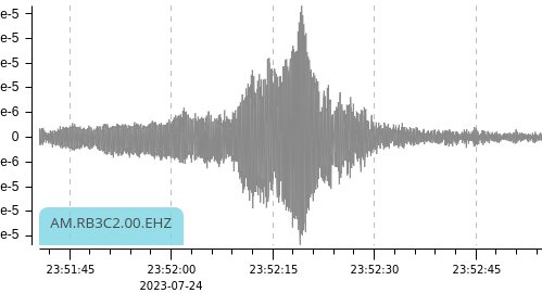 |
 |
| Infrasound | 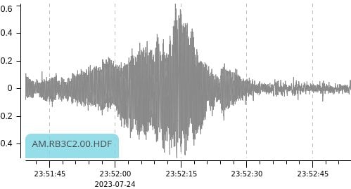 |
 |
The Doppler effect we hear (and see) on RSBs is very similar, and we can ignore most of the differences and other effects related to wind speed and temperature. The biggest differences lie in the math. For the train case, we are most likely to know the frequency of the bell and the speed of the train, and want to determine the frequencies during approach and departure. For RSB users, we can read those frequencies from the spectrum and are interested in the speed of the helicopter. And we’re not at all interested in the fundamental frequency of the helicopter!
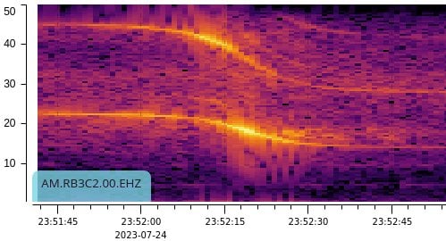
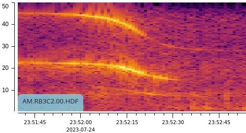
We are somewhat interested in what the helicopter is and what it’s doing – medical and passenger flights are almost always at a constant velocity (speed and direction), police and news helicopters often take odd trajectories, and military flights depend on the mission at hand. Here’s a close look at a Sikorsky Black Hawk helicopter – large, loud, and passing almost overhead. And fast, as we shall see.
The air pressure waves from the rotors have two main sources. One is horizontal – the leading edge of the blades pushes air out of the way. The forward motion of the helicopter adds to the air blade moving forward, but subtracts from it when the blade moves backwards. We hear this primarily as a louder approach than departure. The blades create lift by accelerating air downward and add more complexity to what we hear. The seismic signal is even more complex, and sound waves hit the ground at different angles, and the speed of sound is much higher through the ground than through the air. When the helicopter is overhead, I suspect the seismic signal is at its cleanest and likely explains its more compact envelope.
Of course, none of this is germane to calculating the speed of the helicopter!
We can read the approach and departure frequencies on spectrum plots. The upper line is the first harmonic, and its bigger change allows us to read the higher resolution values, 46 and 27 Hz. It seemed to me there ought to be some simple formula to convert those frequencies into the speed of the helicopter. It turns out that the math and visualization are much easier if we work with the wavelengths of the pulse train. It also helps if we use Mach numbers for speed, as the speed of sound is simply Mach 1.
Geometry: Sound/Pressure Waves and a Moving Source
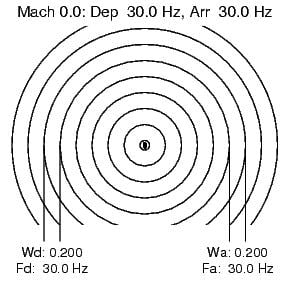
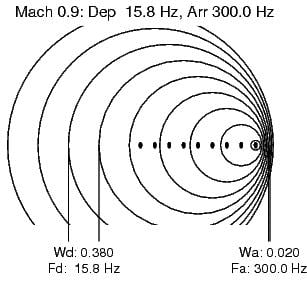
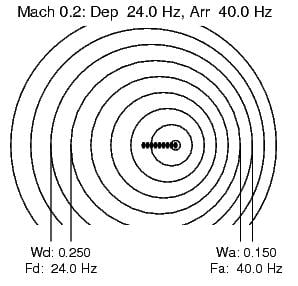
Consider these three cases of a sound source emitting a 30 Hz pulse train:
 |
 |
 |
The first is the source at rest; all waves have a common starting point, and the wavelength, Wd and Ws are the same. (The 0.200 is just the width measured on the plotting software).
The middle plot is near another extreme, Mach 0.90, nearly the speed of sound. The waves in front of the source almost run into each other, and the waves behind the source are nearly twice the original. (Note that Wd + Ws in all three plots is 0.400, but the relationship between the frequencies is not so simple).
The third plot shows a more realistic case where the source, a helicopter, can do this while traveling at Mach 0.25 (The figure’s 0.2 is rounded down).
Algebra: Getting to the Numbers
We need symbols to write equations. First, we’re working with these concepts:
- \( c \): The speed of sound. Physicists seem to like to use \( c \) for both the speed of sound and the speed of light.
- \( v \): Velocity (actually speed) of the source. The observers are at \( 0 \). Note that \( \frac{v}{c} \) is the Mach number.
- \( w \): Wavelengths of the motionless source and those seen by the observers.
- \( f \): Frequencies of the source and heard by the observers. They're just the reciprocal of the related wavelength.
The variables use these subscripts to connect them to the objects:
- \( s \): Source: Not used for velocity as the source is the only one that needs it.
- \( d \): Departure: The observer seeing the source depart.
- \( a \): Arrival: The observer seeing the source arriving.
Here’s how we get from wavelengths to frequencies to speed.
| The wavelengths the observers see depends on the velocity of the source | \(w_d = w_s \times \frac{c + v}{c}\) \(w_a = w_s \times \frac{c - v}{c}\) |
| Solving for \(w_s\) | \(w_s = w_d \times \frac{c}{c + v} = w_a \times \frac{c}{c - v}\) |
| Flipping to start using frequencies | \(f_s = f_d \times \frac{c + v}{c} = f_a \times \frac{c - v}{c}\) |
| Dropping \(f_s\) and that \(c\) | \(f_d(c + v) = f_a(c - v)\) |
| Expanding the multiplication | \(f_d c + f_d v = f_a c - f_a v\) |
| Get just the \(v\) terms on the left | \(f_d v + f_a v = f_a c - f_d c\) |
| Factoring | \(v(f_d + f_a) = c(f_a - f_d)\) |
| Solving for \(v\) yields Rie's equation | \(v = c \times \frac{f_a - f_d}{f_a + f_d}\) |
| In miles per hour | \(v = 760 \times \frac{f_a - f_d}{f_a + f_d}\) |
| In kilometers per hour | \(v = 1225 \times \frac{f_a - f_d}{f_a + f_d}\) |
Note that at small Doppler shifts \(\frac{f_a - f_d}{f_a + f_d}\) will be small and the equation will yield a low speed. At large shifts, \(\frac{f_a - f_d}{f_a + f_d}\) dominates the equation and speed will approach the speed of sound. Simple and elegant, as I hoped.
As for that Helicopter
Above, I noted that the frequency drops from 46 Hz to 27 Hz. Therefore, the speed is:
\(760 \times \frac{46 - 27}{46 + 27} = 198\) mph.
While those frequencies are imprecise, they fit better than I expected. This image from FlightRadar24.com reports 196 mph:

While I did pick this trace for the big difference in frequencies, there’s a bit of a catch. Wikipedia’s Sikorsky UH-60 Black Hawk web page suggests the pilot is in a hurry:
- Maximum speed: 159 kn (183 mph, 294 km/h)
- Cruise speed: 152 kn (175 mph, 282 km/h) maximum range at 18,000 lb
- Never exceed speed: 193 kn (222 mph, 357 km/h)
I don’t have the airspeed, I’ll just assume it had a tailwind. I believe my equation is computing the ground speed – if the air speed equals the headwind’s speed, then the helicopter will be motionless and you’ll hear the source frequency.
Final note
Yes, calling this Ric’s Equation is more than a bit presumptuous. However, after I derived this, I went looking for it on the web – and didn’t find it! Pretty much everything I found applied to the train crossing bell – start with the source velocity and frequency, then derive the frequency the observers would hear. I conclude that before Raspberry Shakes showed up, few people had the frequency data that’s now ours for the picking.