
PLANES, QUAKES AND GEOTHERMAL ACTIVITY GET THINGS SHAKING IN THE SMALL TOWN OF CLOVERDALE
24 June, 2019 – Written by David Fowler
To provide some background, I’m a geologist working for the state of California. I live in a small town called Cloverdale in the middle of northern California’s “Wine Country,” about 125 km (78 mi) north of San Francisco. I’ve been operating a combined Raspberry Shake 3D and 4D for about nine months. In addition, I’ve donated three Raspberry Shake 1Ds to local schools. I enjoy working with students and although I am not a geophysicist, as a geologist I’ve been able to provide some elementary introduction to seismology.
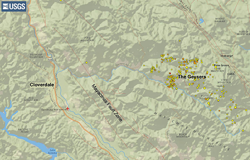
Cloverdale is located between the San Andreas and the Mayacmas fault zones (approximately 35 km (22 mi) west and 6 km (3.7 mi) east, respectively) and is 15 to 25 km (9 to 15 mi) from The Geysers, a seismically active and very well instrumented geothermal area. While there are no actual geysers at The Geysers, it is an area of natural hot springs and a commercial geothermal power generation operation.

Map 1. Cloverdale and The Geysers
On the map image above, the yellow and orange dots are events recorded during the week of March 17 through 23, 2019. The orange dots were recorded in the last 24 hour period (March 23). The number and pattern of events shown is standard for most any given week.

Figure 1. A small swarm of six events within three minutes at The Geysers on May 10, 2018. The events ranged from M 4.2 to less than M 1.0.
Because of the possibility of induced seismic activity due to deep water injection for geothermal power operation, The Geysers report an average of six to 20 seismic events per day to the USGS Earthquake Catalog, although as many as 30 (or more) events in a day is not uncommon. The events recorded at The Geysers are generally small, usually between M 0.2 and M 2.5. For example, during the same seven-day period as the map, from March 17 through 23, 2019, there were 219 events recorded at The Geysers – 172 less than M 1.0, 43 from M 1.0 to M 1.9, and four M 2.0 and greater. Depending on size and distance, about one third of the USGS listed events at The Geysers are detectable by our Raspberry Shakes in Cloverdale. We can usually detect events greater than M 1.5 anywhere at The Geysers (up to 32 km, or 20 miles, distant), but we generally cannot detect events less than M 1.0 unless they are within about 17 km (11 miles).

Figure 2. Magnitude vs. Distance from Cloverdale, California
Figure 2 is a graph of magnitude vs. distance (in degrees arc) of all events detected by my Raspberry Shake 3D during the six months of August 2018 through January 2019. The graph includes non-detectable events within approximately two magnitudes below what we’ve been able to detect in order to show the gradational transition between what is and is not detectable. Events plotted are from both the USGS Earthquake Catalog and Natural Resources Canada, Earthquakes Canada catalog.
We used the USGS SWARM software to determine detectable events. The events shown as “Weakly Detected” on the graph are ones that were difficult to discern, but were subsequently confirmed by the USGS catalog record.
The large concentration of events between approximately 0.12 and 0.25 degrees are mostly from The Geysers. Of the approximately 800 detectable events plotted on the graph, just over 600 are from The Geysers.

Figure 3. PKP and PP arrivals from an M 7.1 event on the East Scotia Ridge, approximately 125 degrees distant.
The gray points on the right side of the graph in Figure 2. are events within the “seismic shadow” greater than 103 degrees arc distance where direct direct seismic waves are blocked (in the case of S-waves) or refracted (in the case of P-Waves) by the Earth’s outer core. We were therefore quite excited to see that the Raspberry Shakes detected two events within the shadow zone. One was an M 7.5 event in Indonesia approximately 111 degrees distant (12,000 km, 7,700 mi). The arrival time matched very closely with the expected PP arrival time. The other was an M 7.1 in the South Sandwich Islands on the East Scotia Ridge approximately 125 degrees distant (14,000 km, 8,700 mi). We detected both the PKP and PP arrivals for that one.

Figure 4. P-wave travel time vs. Distance traveled
Figure 4 is a graph of the P-wave travel time versus distance in degrees arc, based on the event time and location recorded in the USGS Earthquake Catalog and the time the event was detected on our Raspberry Shake in Cloverdale. It includes data for selected events within the three month period from November 2018 through January 2019. We plotted every event greater than 5 degrees distant, but only a very small sample of those less than 5 degrees distant due to the large number of nearby events. The green line is the average P-wave travel time curve from the USGS – not a bad fit! One of the ways I use this graph is to show students that even though the difference between predicted and actual travel times are generally small (remarkably small in most cases), there is some variation – in other words, the Earth is not a homogenous layer-cake.

Figure 5. SWARM helicorder record of the May 4, 2018, M 6.9 earthquake in Hawaii.
Figure 5 is the helicorder record of the May 4, 2018, M 6.9 earthquake in Hawaii. It is quite remarkable and a great record to show to students for several reasons: It shows the difference between nearby small events (M 3.4, 0.53 degrees arc, 58 km, 36 mi), and distant large events (M 6.9, approximately 34 degrees arc, 3,760 km, 2,300 mi); the P-, S-, and surface wave arrivals of the M 6.9 event are very distinct; and the surface waves persist for over two hours. After viewing all three Z, N, and E graphs, and the SWARM particle movement plots, a friend who is an acoustical engineer commented that it looked very similar to the acoustic signature of a large bell. So now I have proof when I tell students earthquakes really do make the Earth ring like a bell!

Figure 6. Seismograms of the May 4, 2018, M 6.9 earthquake in Hawaii.
Figure 6 is from the same M 6.9 event in Hawaii seen in Figure 3, but showing all three Z, N, and E axes. It is one of my favorite charts because the P-, S-, Love, and Rayleigh arrivals are all so distinct. It clearly shows the P-wave arrival is strongest in the vertical record, while the S-wave arrival is strongest in the horizontal (as one would expect). It is also easy to see that while the Love waves are quite strong in the horizontal, they’re nearly absent in the vertical (again, as one would expect). To me, I think it’s quite exciting to see real-world events recorded on the Raspberry Shake that demonstrate principles I’ve previously only read about. It also makes those principles all that much more real and meaningful to students.

Figure 7. Doppler spectrogram.
Shortly after installing my Raspberry Shake, I started noticing events with a peculiar “sigmoidal” spectrogram. At first I wasn’t sure what was causing this particular spectrogram signature. Then one day while I was cataloging detectable events, I happened to hear a propeller airplane fly overhead and noticed the familiar spectrogram recorded by the Raspberry Shake. The spectrogram shows the airplane approaching, the observed frequency dropping due to the Doppler shift as it passes over head, and then receding. I should mention that the (small, single runway) Cloverdale airport is only 6 km away. I have not yet calculated the velocity of the aircraft from the Doppler shift (as described in the October 3, 2018, article by Jean-Paul Arnoul), but I have thought about suggesting it as an exercise for students.
My personal Raspberry Shake’s include the RS3D (AM.R57B0), RS4D (AM.RCCAC) and soon I will be adding the RBOOM. They are currently in the back of an isolated closet in my house, and even though they are as far as they can be from any human or mechanical activity in the house, noise can still be a problem. My next project, therefore, is to create a vault in my backyard along the lines of the USGS Open File Report 02-0144, as referenced in Steve Carson’s November 7, 2018, article.
One last word, I want to say THANK YOU VERY MUCH! to everyone on the Raspberry Shake team for all that they’ve done to create, distribute, update, and support the Raspberry Shake. It is a fantastic combination of hardware and software with many applications, not the least of which is to get young people interested and excited about science in general and earth sciences in particular. Thanks!
From all of us at Raspberry Shake we want to say a BIG thank you to David Fowler for being such an active “Shaker” and kindly sharing his rocking story (pun intended!). We love what we do at Raspberry Shake and our incredible team puts their heart and soul into everyday making things just a little more awesome – Hearing your stories, findings and kind words makes it all worth while!
HAPPY SHAKING!


